2  Data manipulation

All examples in this chapter use a real-world dataset of approximately 530,000 US domestic flights from January 2022.

full_flights = pl.read_csv('./data/On_Time_Reporting_Carrier_On_Time_Performance_(1987_present)_2022_1.csv')
full_flights.shape

(537902, 110)

full_flights.estimated_size('mb')

240.02948379516602

2.1 Data type conversion

The way R and Polars handle types reflects a fundamental design difference: R prioritises convenience through implicit coercion, while Polars prioritises correctness through explicit conversion.

2.1.1 R: implicit type coercion

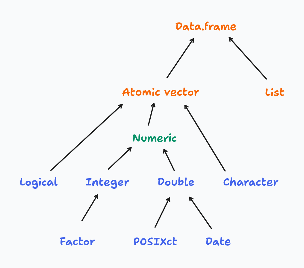
R’s type system is built around four atomic vector types — logical, integer, double, and character — arranged in a coercion hierarchy:

When you combine values of mixed types, R silently promotes them up the hierarchy to find a common type:

# R coerces everything to the "highest" type in the hierarchy
x <- c(TRUE, 1L, 2.5)
typeof(x)  # "double" — logical and integer were silently promoted

y <- c(TRUE, 1L, 2.5, "text")
typeof(y)  # "character" — everything coerced to string

This makes interactive exploration forgiving — R rarely stops you with a type error. The cost is that type mismatches surface as subtly wrong results rather than loud errors, which makes bugs hard to trace in larger codebases.

2.1.2 Polars: explicit type conversion

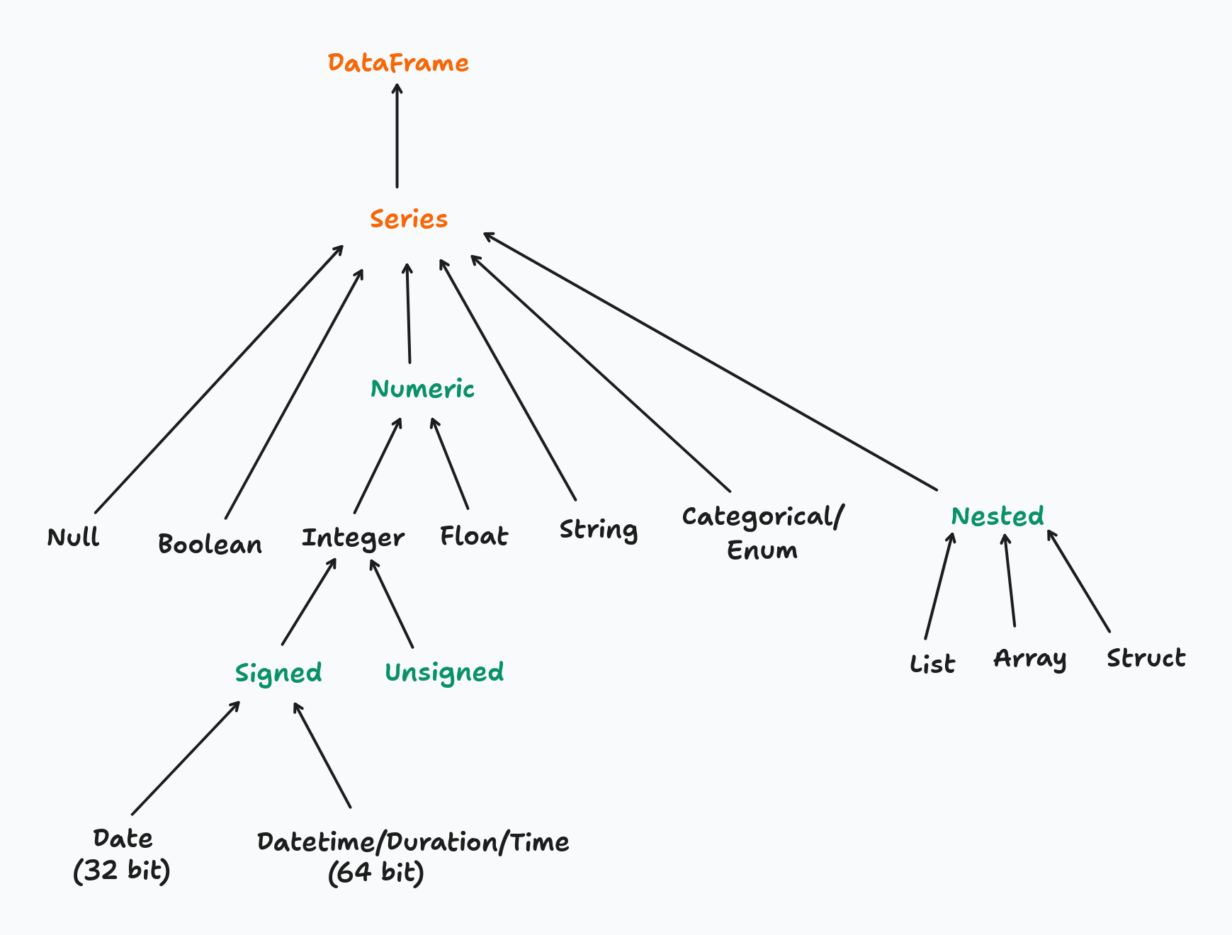
Polars has a much richer type system — granular numeric types (Int8 through Int64, UInt8 through UInt64, Float32, Float64), dedicated temporal types, nested types, and more:

Polars never coerces silently. Every type change must be declared explicitly with .cast(). You can inspect the current type of a column before acting on it:

full_flights['Year'].dtype

Int64

To convert the Year column from integer to string:

full_flights = full_flights.with_columns(
    pl.col('Year').cast(pl.String)
)
full_flights['Year'].dtype

String

If .cast() cannot perform the conversion safely (e.g. casting "abc" to Int64), Polars raises an error immediately rather than producing a null or a wrong value — unless you explicitly opt in to lenient casting with strict=False.

The tradeoff is intentional: explicit casting is more verbose, but type contracts are visible in the code and mistakes fail loudly at the point of conversion. For production pipelines processing millions of rows, catching a type mismatch early is far cheaper than diagnosing a silently incorrect result downstream.

2.2 Introduction to methods

In Python, a method is a function that belongs to an object and is invoked using dot notation: object.method(). The object provides both the data and the set of operations available on it.

The distinction from a standalone function comes down to ownership:

# standalone functions — data is passed as an argument
len(full_flights)
pl.read_csv('./data/flights.csv')

# methods — the object is the implicit first argument
full_flights.shape
full_flights.head()
full_flights.filter(pl.col('OriginStateName') == 'Ohio')

A method always has implicit access to the object it belongs to. A DataFrame method like .filter() knows it is operating on a DataFrame; a Series method like .mean() knows it is operating on a Series. This means methods are type-specific — .filter() exists on a DataFrame but not on a Series.

2.2.1 Comparison with R

R’s tidyverse follows a function-first style: data is passed as the first argument to a verb, and the pipe operator chains those verbs into a pipeline:

# R / dplyr: functions act on data passed as an argument
full_flights |>
    filter(OriginStateName == 'Ohio') |>
    select(FlightDate, Origin, Dest)

Python/Polars follows a method chaining style: the data object comes first, and methods are applied sequentially via the dot operator:

(
    full_flights
    .filter(pl.col('OriginStateName') == 'Ohio')
    .select(['FlightDate', 'Origin', 'Dest'])
)

The two patterns are structurally equivalent — both read as a left-to-right pipeline of transformations. The key difference is where the data lives: in R, data flows through functions as an argument; in Python, data is the object and methods are behaviors it carries with it.

One practical consequence of this is that in R, filter() works on any compatible object — data frames, tibbles, grouped tibbles. In Python, each type exposes its own set of methods, so you need to be aware of what type you are working with at each step of the chain.

2.3 Single table operation

2.3.1 Filtering rows

Filtering rows in Polars maps directly to dplyr’s filter(). The function name is the same; the main syntax difference is that Polars requires column references to be wrapped in pl.col().

• Retrieving all flights from Ohio (filtering based on one condition):

# dplyr
flights_from_ohio <- full_flights |> filter(OriginStateName == "Ohio")

flights_from_ohio = full_flights.filter(pl.col('OriginStateName') == 'Ohio')
flights_from_ohio.shape

(7434, 110)

• Filtering based on multiple conditions:

# dplyr — comma-separated predicates are implicitly AND-ed
flights_from_ohio_to_virginia <- full_flights |>
    filter(OriginStateName == "Ohio", DestStateName == "Virginia")

# note that each predicate must be enclosed within parentheses when using &
flights_from_ohio_to_virginia = full_flights.filter(
    (pl.col('OriginStateName') == 'Ohio') & (pl.col('DestStateName') == 'Virginia')
)

# comma-separated predicates are also AND-ed, avoiding the need for parentheses
# flights_from_ohio_to_virginia = full_flights.filter(
#     pl.col('OriginStateName') == 'Ohio',
#     pl.col('DestStateName') == 'Virginia'
# )

flights_from_ohio_to_virginia.shape

(564, 110)

• Filtering with a negative condition:

# dplyr
flights_from_ohio_except_virginia <- full_flights |>
    filter(OriginStateName == "Ohio", DestStateName != "Virginia")

flights_from_ohio_except_virginia = full_flights.filter(
    pl.col('OriginStateName') == 'Ohio',
    ~(pl.col('DestStateName') == 'Virginia')
)
flights_from_ohio_except_virginia.shape

(6870, 110)

• Filtering with a set of values using .is_in(), the equivalent of R’s %in% operator:

# dplyr
major_hubs <- full_flights |>
    filter(OriginStateName %in% c("California", "Texas", "New York"))

major_hubs = full_flights.filter(
    pl.col('OriginStateName').is_in(['California', 'Texas', 'New York'])
)
major_hubs.shape

(143765, 110)

• Why prefer .filter() over boolean indexing (df[df['col'] == value])? .filter() integrates with Polars’ lazy execution engine: when used with scan_csv() or scan_parquet(), the predicate is pushed down to the file scan so only qualifying rows are ever read from disk. Boolean indexing always loads the full dataset first. See the Lazy API chapter for a detailed benchmark.

2.3.2 Selecting columns

Polars offers three levels of column selection, progressing from explicit to declarative:

1. By name — a string list; simple but brittle if column names change
2. By type — pl.col(dtype) selects all columns of a given type
3. Selectors (polars.selectors) — a high-level API for flexible, composable selection based on types, name patterns, or properties

Selectors are the recommended approach for anything beyond a simple name list. They produce code that reads closer to intent, composes naturally with set operations, and adapts automatically when the schema changes.

2.3.2.1 Selecting by name

# dplyr
full_flights |> select(FlightDate, Tail_Number)

full_flights.select(['FlightDate', 'Tail_Number']).head(3)

shape: (3, 2)

FlightDate	Tail_Number
str	str
"2022-01-14"	"N119HQ"
"2022-01-15"	"N122HQ"
"2022-01-16"	"N412YX"

2.3.2.2 Selecting by type

pl.col(dtype) selects all columns that match a given type. Useful for applying the same transformation to every column of a type:

# dplyr
full_flights |> select(where(is.double))
full_flights |> select(where(is.integer))

full_flights.select(pl.col(pl.Float64)).head(3)

shape: (3, 22)

DepDelay	DepDelayMinutes	DepDel15	TaxiOut	TaxiIn	ArrDelay	ArrDelayMinutes	ArrDel15	Cancelled	Diverted	CRSElapsedTime	ActualElapsedTime	AirTime	Flights	Distance	CarrierDelay	WeatherDelay	NASDelay	SecurityDelay	LateAircraftDelay	TotalAddGTime	LongestAddGTime
f64	f64	f64	f64	f64	f64	f64	f64	f64	f64	f64	f64	f64	f64	f64	f64	f64	f64	f64	f64	f64	f64
-3.0	0.0	0.0	28.0	4.0	4.0	4.0	0.0	0.0	0.0	88.0	95.0	63.0	1.0	323.0	null	null	null	null	null	null	null
-10.0	0.0	0.0	19.0	5.0	-24.0	0.0	0.0	0.0	0.0	88.0	74.0	50.0	1.0	323.0	null	null	null	null	null	null	null
-6.0	0.0	0.0	16.0	12.0	-13.0	0.0	0.0	0.0	0.0	88.0	81.0	53.0	1.0	323.0	null	null	null	null	null	null	null

full_flights.select(pl.col(pl.Int64)).head(3)

shape: (3, 22)

Quarter	Month	DayofMonth	DayOfWeek	DOT_ID_Reporting_Airline	Flight_Number_Reporting_Airline	OriginAirportID	OriginAirportSeqID	OriginCityMarketID	OriginStateFips	OriginWac	DestAirportID	DestAirportSeqID	DestCityMarketID	DestStateFips	DestWac	CRSDepTime	DepartureDelayGroups	CRSArrTime	ArrivalDelayGroups	DistanceGroup	DivAirportLandings
i64	i64	i64	i64	i64	i64	i64	i64	i64	i64	i64	i64	i64	i64	i64	i64	i64	i64	i64	i64	i64	i64
1	1	14	5	20452	4879	11066	1106606	31066	39	44	11278	1127805	30852	51	38	1224	-1	1352	0	2	0
1	1	15	6	20452	4879	11066	1106606	31066	39	44	11278	1127805	30852	51	38	1224	-1	1352	-2	2	0
1	1	16	7	20452	4879	11066	1106606	31066	39	44	11278	1127805	30852	51	38	1224	-1	1352	-1	2	0

2.3.2.3 Selecting with Selectors

polars.selectors provides a declarative selection API that closely mirrors dplyr’s selection helpers. Import it as cs by convention:

import polars.selectors as cs

Select by data type:

# dplyr
full_flights |> select(where(is.numeric))
full_flights |> select(where(is.character))

full_flights.select(cs.numeric()).head(3)  # all Int*, UInt*, Float* columns

shape: (3, 44)

Quarter	Month	DayofMonth	DayOfWeek	DOT_ID_Reporting_Airline	Flight_Number_Reporting_Airline	OriginAirportID	OriginAirportSeqID	OriginCityMarketID	OriginStateFips	OriginWac	DestAirportID	DestAirportSeqID	DestCityMarketID	DestStateFips	DestWac	CRSDepTime	DepDelay	DepDelayMinutes	DepDel15	DepartureDelayGroups	TaxiOut	TaxiIn	CRSArrTime	ArrDelay	ArrDelayMinutes	ArrDel15	ArrivalDelayGroups	Cancelled	Diverted	CRSElapsedTime	ActualElapsedTime	AirTime	Flights	Distance	DistanceGroup	CarrierDelay	WeatherDelay	NASDelay	SecurityDelay	LateAircraftDelay	TotalAddGTime	LongestAddGTime	DivAirportLandings
i64	i64	i64	i64	i64	i64	i64	i64	i64	i64	i64	i64	i64	i64	i64	i64	i64	f64	f64	f64	i64	f64	f64	i64	f64	f64	f64	i64	f64	f64	f64	f64	f64	f64	f64	i64	f64	f64	f64	f64	f64	f64	f64	i64
1	1	14	5	20452	4879	11066	1106606	31066	39	44	11278	1127805	30852	51	38	1224	-3.0	0.0	0.0	-1	28.0	4.0	1352	4.0	4.0	0.0	0	0.0	0.0	88.0	95.0	63.0	1.0	323.0	2	null	null	null	null	null	null	null	0
1	1	15	6	20452	4879	11066	1106606	31066	39	44	11278	1127805	30852	51	38	1224	-10.0	0.0	0.0	-1	19.0	5.0	1352	-24.0	0.0	0.0	-2	0.0	0.0	88.0	74.0	50.0	1.0	323.0	2	null	null	null	null	null	null	null	0
1	1	16	7	20452	4879	11066	1106606	31066	39	44	11278	1127805	30852	51	38	1224	-6.0	0.0	0.0	-1	16.0	12.0	1352	-13.0	0.0	0.0	-1	0.0	0.0	88.0	81.0	53.0	1.0	323.0	2	null	null	null	null	null	null	null	0

full_flights.select(cs.string()).head(3)   # all String columns

shape: (3, 66)

Year	FlightDate	Reporting_Airline	IATA_CODE_Reporting_Airline	Tail_Number	Origin	OriginCityName	OriginState	OriginStateName	Dest	DestCityName	DestState	DestStateName	DepTime	DepTimeBlk	WheelsOff	WheelsOn	ArrTime	ArrTimeBlk	CancellationCode	FirstDepTime	DivReachedDest	DivActualElapsedTime	DivArrDelay	DivDistance	Div1Airport	Div1AirportID	Div1AirportSeqID	Div1WheelsOn	Div1TotalGTime	Div1LongestGTime	Div1WheelsOff	Div1TailNum	Div2Airport	Div2AirportID	Div2AirportSeqID	Div2WheelsOn	Div2TotalGTime	Div2LongestGTime	Div2WheelsOff	Div2TailNum	Div3Airport	Div3AirportID	Div3AirportSeqID	Div3WheelsOn	Div3TotalGTime	Div3LongestGTime	Div3WheelsOff	Div3TailNum	Div4Airport	Div4AirportID	Div4AirportSeqID	Div4WheelsOn	Div4TotalGTime	Div4LongestGTime	Div4WheelsOff	Div4TailNum	Div5Airport	Div5AirportID	Div5AirportSeqID	Div5WheelsOn	Div5TotalGTime	Div5LongestGTime	Div5WheelsOff	Div5TailNum
str	str	str	str	str	str	str	str	str	str	str	str	str	str	str	str	str	str	str	str	str	str	str	str	str	str	str	str	str	str	str	str	str	str	str	str	str	str	str	str	str	str	str	str	str	str	str	str	str	str	str	str	str	str	str	str	str	str	str	str	str	str	str	str	str	str
"2022"	"2022-01-14"	"YX"	"YX"	"N119HQ"	"CMH"	"Columbus, OH"	"OH"	"Ohio"	"DCA"	"Washington, DC"	"VA"	"Virginia"	"1221"	"1200-1259"	"1249"	"1352"	"1356"	"1300-1359"	""	""	null	null	null	null	""	null	null	""	null	null	""	""	""	null	null	""	null	null	""	""	""	null	null	""	null	null	""	""	""	null	null	""	null	null	""	""	""	null	null	""	null	null	""	""	null
"2022"	"2022-01-15"	"YX"	"YX"	"N122HQ"	"CMH"	"Columbus, OH"	"OH"	"Ohio"	"DCA"	"Washington, DC"	"VA"	"Virginia"	"1214"	"1200-1259"	"1233"	"1323"	"1328"	"1300-1359"	""	""	null	null	null	null	""	null	null	""	null	null	""	""	""	null	null	""	null	null	""	""	""	null	null	""	null	null	""	""	""	null	null	""	null	null	""	""	""	null	null	""	null	null	""	""	null
"2022"	"2022-01-16"	"YX"	"YX"	"N412YX"	"CMH"	"Columbus, OH"	"OH"	"Ohio"	"DCA"	"Washington, DC"	"VA"	"Virginia"	"1218"	"1200-1259"	"1234"	"1327"	"1339"	"1300-1359"	""	""	null	null	null	null	""	null	null	""	null	null	""	""	""	null	null	""	null	null	""	""	""	null	null	""	null	null	""	""	""	null	null	""	null	null	""	""	""	null	null	""	null	null	""	""	null

Select by name pattern:

# dplyr
full_flights |> select(starts_with("Flight"))
full_flights |> select(ends_with("Delay"))

full_flights.select(cs.starts_with('Flight')).head(3)

shape: (3, 3)

FlightDate	Flight_Number_Reporting_Airline	Flights
str	i64	f64
"2022-01-14"	4879	1.0
"2022-01-15"	4879	1.0
"2022-01-16"	4879	1.0

full_flights.select(cs.ends_with('Delay')).head(3)

shape: (3, 8)

DepDelay	ArrDelay	CarrierDelay	WeatherDelay	NASDelay	SecurityDelay	LateAircraftDelay	DivArrDelay
f64	f64	f64	f64	f64	f64	f64	str
-3.0	4.0	null	null	null	null	null	null
-10.0	-24.0	null	null	null	null	null	null
-6.0	-13.0	null	null	null	null	null	null

Combining selectors with set operations:

This is where selectors go beyond what bare pl.col() can express. Selectors support set operations using Python operators, making complex multi-criteria selections readable in a single expression:

operator	meaning	dplyr equivalent
|	union — columns matching either selector	c(starts_with(), ...)
&	intersection — columns matching both selectors	where(\(x) ... & ...)
-	difference — left selector minus right	not available
~	complement — all columns not matching	!selector

# union: columns starting with "Flight" OR ending with "Delay"
full_flights.select(cs.starts_with('Flight') | cs.ends_with('Delay')).head(3)

shape: (3, 11)

FlightDate	Flight_Number_Reporting_Airline	DepDelay	ArrDelay	Flights	CarrierDelay	WeatherDelay	NASDelay	SecurityDelay	LateAircraftDelay	DivArrDelay
str	i64	f64	f64	f64	f64	f64	f64	f64	f64	str
"2022-01-14"	4879	-3.0	4.0	1.0	null	null	null	null	null	null
"2022-01-15"	4879	-10.0	-24.0	1.0	null	null	null	null	null	null
"2022-01-16"	4879	-6.0	-13.0	1.0	null	null	null	null	null	null

# difference: numeric columns excluding Int64 (i.e. Float columns only)
full_flights.select(cs.numeric() - cs.integer()).head(3)

shape: (3, 22)

DepDelay	DepDelayMinutes	DepDel15	TaxiOut	TaxiIn	ArrDelay	ArrDelayMinutes	ArrDel15	Cancelled	Diverted	CRSElapsedTime	ActualElapsedTime	AirTime	Flights	Distance	CarrierDelay	WeatherDelay	NASDelay	SecurityDelay	LateAircraftDelay	TotalAddGTime	LongestAddGTime
f64	f64	f64	f64	f64	f64	f64	f64	f64	f64	f64	f64	f64	f64	f64	f64	f64	f64	f64	f64	f64	f64
-3.0	0.0	0.0	28.0	4.0	4.0	4.0	0.0	0.0	0.0	88.0	95.0	63.0	1.0	323.0	null	null	null	null	null	null	null
-10.0	0.0	0.0	19.0	5.0	-24.0	0.0	0.0	0.0	0.0	88.0	74.0	50.0	1.0	323.0	null	null	null	null	null	null	null
-6.0	0.0	0.0	16.0	12.0	-13.0	0.0	0.0	0.0	0.0	88.0	81.0	53.0	1.0	323.0	null	null	null	null	null	null	null

# complement: everything except string columns
full_flights.select(~cs.string()).head(3)

shape: (3, 44)

Quarter	Month	DayofMonth	DayOfWeek	DOT_ID_Reporting_Airline	Flight_Number_Reporting_Airline	OriginAirportID	OriginAirportSeqID	OriginCityMarketID	OriginStateFips	OriginWac	DestAirportID	DestAirportSeqID	DestCityMarketID	DestStateFips	DestWac	CRSDepTime	DepDelay	DepDelayMinutes	DepDel15	DepartureDelayGroups	TaxiOut	TaxiIn	CRSArrTime	ArrDelay	ArrDelayMinutes	ArrDel15	ArrivalDelayGroups	Cancelled	Diverted	CRSElapsedTime	ActualElapsedTime	AirTime	Flights	Distance	DistanceGroup	CarrierDelay	WeatherDelay	NASDelay	SecurityDelay	LateAircraftDelay	TotalAddGTime	LongestAddGTime	DivAirportLandings
i64	i64	i64	i64	i64	i64	i64	i64	i64	i64	i64	i64	i64	i64	i64	i64	i64	f64	f64	f64	i64	f64	f64	i64	f64	f64	f64	i64	f64	f64	f64	f64	f64	f64	f64	i64	f64	f64	f64	f64	f64	f64	f64	i64
1	1	14	5	20452	4879	11066	1106606	31066	39	44	11278	1127805	30852	51	38	1224	-3.0	0.0	0.0	-1	28.0	4.0	1352	4.0	4.0	0.0	0	0.0	0.0	88.0	95.0	63.0	1.0	323.0	2	null	null	null	null	null	null	null	0
1	1	15	6	20452	4879	11066	1106606	31066	39	44	11278	1127805	30852	51	38	1224	-10.0	0.0	0.0	-1	19.0	5.0	1352	-24.0	0.0	0.0	-2	0.0	0.0	88.0	74.0	50.0	1.0	323.0	2	null	null	null	null	null	null	null	0
1	1	16	7	20452	4879	11066	1106606	31066	39	44	11278	1127805	30852	51	38	1224	-6.0	0.0	0.0	-1	16.0	12.0	1352	-13.0	0.0	0.0	-1	0.0	0.0	88.0	81.0	53.0	1.0	323.0	2	null	null	null	null	null	null	null	0

A full comparison between dplyr and Polars selection features:

dplyr action	dplyr function	polars selector
matches all columns	everything()	cs.all()
matches all numeric columns	where(is.numeric)	cs.numeric()
matches all integer columns	where(is.integer)	cs.integer()
matches all float columns	where(is.double)	cs.float()
matches all string columns	where(is.character)	cs.string()
matches all factor/categorical columns	where(is.factor)	cs.categorical()
matches all date columns	where(\(x) class(x) == "Date")	cs.date()
matches all datetime columns	not available	cs.datetime()
matches all time columns	not available	cs.time()
matches all temporal columns	not available	cs.temporal()
select the last column	last_col()	cs.last()
starts with a prefix	starts_with()	cs.starts_with()
ends with a suffix	ends_with()	cs.ends_with()
contains a literal string	contains()	cs.contains()
matches a regular expression	matches()	cs.matches()
complement of a selection	!selector	~selector
difference between selections	not available	cs_a - cs_b
range of consecutive columns	col1:col10	not available
any of a list, ignoring missing names	any_of()	not available

The full list of selector functions is available in the Polars selectors reference.

2.3.3 Modifying, renaming, and removing columns

2.3.3.1 Adding and modifying columns

with_columns() is the Polars equivalent of dplyr’s mutate(). It adds new columns or overwrites existing ones and returns a new DataFrame:

# dplyr
full_flights |>
    mutate(
        DepDelay_hrs = DepDelay / 60,
        IsDelayed    = DepDelay > 0
    )

(
    full_flights
    .with_columns(
        DepDelay_hrs = pl.col('DepDelay') / 60,
        IsDelayed    = pl.col('DepDelay') > 0
    )
    .select(['FlightDate', 'DepDelay', 'DepDelay_hrs', 'IsDelayed'])
    .head(3)
)

shape: (3, 4)

FlightDate	DepDelay	DepDelay_hrs	IsDelayed
str	f64	f64	bool
"2022-01-14"	-3.0	-0.05	false
"2022-01-15"	-10.0	-0.166667	false
"2022-01-16"	-6.0	-0.1	false

Overwriting an existing column uses the same syntax — assigning to a name that already exists replaces it:

# overwrite DepDelay from Float64 to Int32
full_flights.with_columns(
    pl.col('DepDelay').cast(pl.Int32)
)['DepDelay'].dtype

Int32

2.3.3.2 Parallel execution

A key difference from dplyr is that all expressions inside a single with_columns() call are evaluated in parallel against the original DataFrame. This means you cannot reference a column created earlier in the same call:

# dplyr: works — mutate() evaluates expressions sequentially
full_flights |>
    mutate(
        DepDelay_hrs = DepDelay / 60,
        IsLongDelay  = DepDelay_hrs > 2   # references the column just created above
    )

# Polars: fails — DepDelay_hrs does not exist in the original DataFrame yet
full_flights.with_columns(
    DepDelay_hrs = pl.col('DepDelay') / 60,
    IsLongDelay  = pl.col('DepDelay_hrs') > 2   # ColumnNotFoundError
)

The fix is to split into two chained with_columns() calls:

(
    full_flights
    .with_columns(DepDelay_hrs = pl.col('DepDelay') / 60)
    .with_columns(IsLongDelay  = pl.col('DepDelay_hrs') > 2)
    .select(['FlightDate', 'DepDelay', 'DepDelay_hrs', 'IsLongDelay'])
    .head(3)
)

shape: (3, 4)

FlightDate	DepDelay	DepDelay_hrs	IsLongDelay
str	f64	f64	bool
"2022-01-14"	-3.0	-0.05	false
"2022-01-15"	-10.0	-0.166667	false
"2022-01-16"	-6.0	-0.1	false

The parallel evaluation is intentional — it allows Polars to optimise multi-column mutations, which is a meaningful performance advantage for wide DataFrames.

2.3.3.3 Renaming columns

.rename() takes a dictionary mapping old names to new names:

# dplyr — note the order: new_name = old_name
full_flights |> rename(departure_delay = DepDelay, arrival_delay = ArrDelay)

# Polars dict order is the reverse: old_name -> new_name
(
    full_flights
    .rename({'DepDelay': 'departure_delay', 'ArrDelay': 'arrival_delay'})
    .select(['FlightDate', 'departure_delay', 'arrival_delay'])
    .head(3)
)

shape: (3, 3)

FlightDate	departure_delay	arrival_delay
str	f64	f64
"2022-01-14"	-3.0	4.0
"2022-01-15"	-10.0	-24.0
"2022-01-16"	-6.0	-13.0

Note the reversed convention: dplyr uses new_name = old_name, while Polars maps old_name → new_name.

2.3.3.4 Removing columns

.drop() removes one or more columns by name:

# dplyr
full_flights |> select(-Year, -Quarter)

full_flights.drop(['Year', 'Quarter']).head(3)

shape: (3, 108)

Month	DayofMonth	DayOfWeek	FlightDate	Reporting_Airline	DOT_ID_Reporting_Airline	IATA_CODE_Reporting_Airline	Tail_Number	Flight_Number_Reporting_Airline	OriginAirportID	OriginAirportSeqID	OriginCityMarketID	Origin	OriginCityName	OriginState	OriginStateFips	OriginStateName	OriginWac	DestAirportID	DestAirportSeqID	DestCityMarketID	Dest	DestCityName	DestState	DestStateFips	DestStateName	DestWac	CRSDepTime	DepTime	DepDelay	DepDelayMinutes	DepDel15	DepartureDelayGroups	DepTimeBlk	TaxiOut	WheelsOff	WheelsOn	…	Div1TotalGTime	Div1LongestGTime	Div1WheelsOff	Div1TailNum	Div2Airport	Div2AirportID	Div2AirportSeqID	Div2WheelsOn	Div2TotalGTime	Div2LongestGTime	Div2WheelsOff	Div2TailNum	Div3Airport	Div3AirportID	Div3AirportSeqID	Div3WheelsOn	Div3TotalGTime	Div3LongestGTime	Div3WheelsOff	Div3TailNum	Div4Airport	Div4AirportID	Div4AirportSeqID	Div4WheelsOn	Div4TotalGTime	Div4LongestGTime	Div4WheelsOff	Div4TailNum	Div5Airport	Div5AirportID	Div5AirportSeqID	Div5WheelsOn	Div5TotalGTime	Div5LongestGTime	Div5WheelsOff	Div5TailNum
i64	i64	i64	str	str	i64	str	str	i64	i64	i64	i64	str	str	str	i64	str	i64	i64	i64	i64	str	str	str	i64	str	i64	i64	str	f64	f64	f64	i64	str	f64	str	str	…	str	str	str	str	str	str	str	str	str	str	str	str	str	str	str	str	str	str	str	str	str	str	str	str	str	str	str	str	str	str	str	str	str	str	str	str	str
1	14	5	"2022-01-14"	"YX"	20452	"YX"	"N119HQ"	4879	11066	1106606	31066	"CMH"	"Columbus, OH"	"OH"	39	"Ohio"	44	11278	1127805	30852	"DCA"	"Washington, DC"	"VA"	51	"Virginia"	38	1224	"1221"	-3.0	0.0	0.0	-1	"1200-1259"	28.0	"1249"	"1352"	…	null	null	""	""	""	null	null	""	null	null	""	""	""	null	null	""	null	null	""	""	""	null	null	""	null	null	""	""	""	null	null	""	null	null	""	""	null
1	15	6	"2022-01-15"	"YX"	20452	"YX"	"N122HQ"	4879	11066	1106606	31066	"CMH"	"Columbus, OH"	"OH"	39	"Ohio"	44	11278	1127805	30852	"DCA"	"Washington, DC"	"VA"	51	"Virginia"	38	1224	"1214"	-10.0	0.0	0.0	-1	"1200-1259"	19.0	"1233"	"1323"	…	null	null	""	""	""	null	null	""	null	null	""	""	""	null	null	""	null	null	""	""	""	null	null	""	null	null	""	""	""	null	null	""	null	null	""	""	null
1	16	7	"2022-01-16"	"YX"	20452	"YX"	"N412YX"	4879	11066	1106606	31066	"CMH"	"Columbus, OH"	"OH"	39	"Ohio"	44	11278	1127805	30852	"DCA"	"Washington, DC"	"VA"	51	"Virginia"	38	1224	"1218"	-6.0	0.0	0.0	-1	"1200-1259"	16.0	"1234"	"1327"	…	null	null	""	""	""	null	null	""	null	null	""	""	""	null	null	""	null	null	""	""	""	null	null	""	null	null	""	""	""	null	null	""	null	null	""	""	null

To remove columns by type or name pattern, use .select() with a selector complement instead:

# remove all string columns
full_flights.select(~cs.string()).head(3)

shape: (3, 44)

Quarter	Month	DayofMonth	DayOfWeek	DOT_ID_Reporting_Airline	Flight_Number_Reporting_Airline	OriginAirportID	OriginAirportSeqID	OriginCityMarketID	OriginStateFips	OriginWac	DestAirportID	DestAirportSeqID	DestCityMarketID	DestStateFips	DestWac	CRSDepTime	DepDelay	DepDelayMinutes	DepDel15	DepartureDelayGroups	TaxiOut	TaxiIn	CRSArrTime	ArrDelay	ArrDelayMinutes	ArrDel15	ArrivalDelayGroups	Cancelled	Diverted	CRSElapsedTime	ActualElapsedTime	AirTime	Flights	Distance	DistanceGroup	CarrierDelay	WeatherDelay	NASDelay	SecurityDelay	LateAircraftDelay	TotalAddGTime	LongestAddGTime	DivAirportLandings
i64	i64	i64	i64	i64	i64	i64	i64	i64	i64	i64	i64	i64	i64	i64	i64	i64	f64	f64	f64	i64	f64	f64	i64	f64	f64	f64	i64	f64	f64	f64	f64	f64	f64	f64	i64	f64	f64	f64	f64	f64	f64	f64	i64
1	1	14	5	20452	4879	11066	1106606	31066	39	44	11278	1127805	30852	51	38	1224	-3.0	0.0	0.0	-1	28.0	4.0	1352	4.0	4.0	0.0	0	0.0	0.0	88.0	95.0	63.0	1.0	323.0	2	null	null	null	null	null	null	null	0
1	1	15	6	20452	4879	11066	1106606	31066	39	44	11278	1127805	30852	51	38	1224	-10.0	0.0	0.0	-1	19.0	5.0	1352	-24.0	0.0	0.0	-2	0.0	0.0	88.0	74.0	50.0	1.0	323.0	2	null	null	null	null	null	null	null	0
1	1	16	7	20452	4879	11066	1106606	31066	39	44	11278	1127805	30852	51	38	1224	-6.0	0.0	0.0	-1	16.0	12.0	1352	-13.0	0.0	0.0	-1	0.0	0.0	88.0	81.0	53.0	1.0	323.0	2	null	null	null	null	null	null	null	0

2.3.4 Aggregation by group

Most analytical questions about groups of data follow a common pattern: divide the data into subsets based on one or more keys, apply a function to each subset independently, and reassemble the results. Wickham (2011) formalised this as the split-apply-combine strategy — the conceptual backbone behind group_by() in dplyr, Polars’ group_by() context, and pandas’ groupby().

The strategy has three steps:

1. Split — partition rows into groups based on one or more grouping expressions
2. Apply — compute a summary or transformation independently within each group
3. Combine — assemble the per-group results into a single output

2.3.4.1 Implementation: grouped_df vs GroupBy

dplyr and Polars implement the split-apply-combine strategy differently, and understanding the difference prevents a whole class of subtle bugs.

dplyr wraps the data frame in a grouped_df object. The groups are sticky — they persist across the pipe and silently alter the behaviour of any subsequent verb until you call ungroup():

by_carrier <- full_flights |> group_by(Reporting_Airline)
class(by_carrier)
# "grouped_df" "tbl_df" "tbl" "data.frame"

by_carrier |> summarise(n = n(), mean_delay = mean(DepDelay, na.rm = TRUE))

by_carrier |> ungroup()  # explicitly remove grouping when done

Polars returns a GroupBy object from group_by() — not a DataFrame. The primary operation on a GroupBy is .agg(), which accepts one or more aggregating expressions. The object also exposes:

• Convenience aggregation shortcuts — .len(), .sum(), .mean(), .min(), .max(), .first(), .last(), and others — each equivalent to calling .agg() with the corresponding expression
• .map_groups(fn) — applies a custom Python function to each group’s sub-DataFrame and concatenates the results; useful when the transformation cannot be expressed as a Polars expression
• .having(*predicates) — filters groups by a predicate before aggregation, equivalent to SQL’s HAVING clause

There is no sticky state: each group_by() call is self-contained:

type(full_flights.group_by('Reporting_Airline'))

polars.dataframe.group_by.GroupBy

This design eliminates the class of bugs where a forgotten ungroup() causes downstream verbs to silently operate group-by-group. In Polars, grouping context is always explicit and local to a single expression.

2.3.4.2 Basic aggregation

The fundamental pattern in Polars is group_by() followed by .agg(). Multiple aggregations are passed as comma-separated keyword arguments:

# dplyr
full_flights |>
    group_by(Reporting_Airline) |>
    summarise(
        n_flights  = n(),
        mean_delay = mean(DepDelay, na.rm = TRUE),
        max_delay  = max(DepDelay, na.rm = TRUE)
    )

(
    full_flights
    .group_by('Reporting_Airline')
    .agg(
        n_flights  = pl.len(),
        mean_delay = pl.col('DepDelay').mean(),
        max_delay  = pl.col('DepDelay').max()
    )
    .sort('Reporting_Airline')
)

shape: (17, 4)

Reporting_Airline	n_flights	mean_delay	max_delay
str	u32	f64	f64
"9E"	21644	8.163106	1111.0
"AA"	69400	7.928395	2512.0
"AS"	16549	8.076828	826.0
"B6"	21332	23.401837	1661.0
"DL"	68963	7.864645	1164.0
…	…	…	…
"QX"	8105	12.158578	530.0
"UA"	45741	13.073434	1436.0
"WN"	97436	10.244393	479.0
"YV"	11404	18.966965	1224.0
"YX"	27261	6.944988	1282.0

pl.len() counts rows in each group, equivalent to dplyr’s n(). The .sort() call is necessary because group_by() in Polars does not guarantee output order — dplyr’s summarise() preserves group key order by default.

To group by multiple columns, pass a list:

# dplyr
full_flights |>
    group_by(Reporting_Airline, OriginStateName) |>
    summarise(n_flights = n(), mean_delay = mean(DepDelay, na.rm = TRUE))

(
    full_flights
    .group_by(['Reporting_Airline', 'OriginStateName'])
    .agg(
        n_flights  = pl.len(),
        mean_delay = pl.col('DepDelay').mean()
    )
    .sort(['Reporting_Airline', 'OriginStateName'])
    .head(10)
)

shape: (10, 4)

Reporting_Airline	OriginStateName	n_flights	mean_delay
str	str	u32	f64
"9E"	"Alabama"	391	4.720627
"9E"	"Arkansas"	91	0.735632
"9E"	"Florida"	138	15.873134
"9E"	"Georgia"	3931	5.657929
"9E"	"Illinois"	420	8.204938
"9E"	"Indiana"	405	6.776923
"9E"	"Iowa"	398	9.82398
"9E"	"Kansas"	7	3.0
"9E"	"Kentucky"	878	7.736277
"9E"	"Louisiana"	387	6.656085

Polars also lets you apply the same aggregation to multiple columns in a single expression using a multi-column selector and .name.suffix() to auto-generate output names — a feature with no direct dplyr equivalent:

# compute mean of all three delay-component columns in one expression
(
    full_flights
    .group_by('Reporting_Airline')
    .agg(
        pl.col('DepDelay', 'ArrDelay', 'CarrierDelay').mean().name.suffix('_mean')
    )
    .sort('Reporting_Airline')
    .head(5)
)

shape: (5, 4)

Reporting_Airline	DepDelay_mean	ArrDelay_mean	CarrierDelay_mean
str	f64	f64	f64
"9E"	8.163106	1.984254	28.540738
"AA"	7.928395	-1.075832	34.993137
"AS"	8.076828	5.233294	21.212693
"B6"	23.401837	18.721082	40.458421
"DL"	7.864645	-0.228486	34.6591

2.3.4.3 How dplyr verbs change behaviour on grouped data

One of dplyr’s defining features is that the same verb produces different output depending on whether grouping is active. The three most important cases are summarise(), mutate(), and filter().

summarise() reduces each group to one row — the familiar aggregation pattern shown above. Polars’ group_by().agg() is the direct equivalent.

Grouped mutate() computes within-group window statistics, keeping all rows intact:

# dplyr: add each carrier's average delay back to every flight row
full_flights |>
    group_by(Reporting_Airline) |>
    mutate(carrier_avg_delay = mean(DepDelay, na.rm = TRUE))
# → same number of rows; new column has the group mean repeated per row

Polars handles this with the .over() window function applied inside .with_columns(). Rather than grouping the DataFrame, .over() computes a group-level aggregate and broadcasts the result back to each row:

(
    full_flights
    .with_columns(
        carrier_avg_delay = pl.col('DepDelay').mean().over('Reporting_Airline')
    )
    .select(['FlightDate', 'Reporting_Airline', 'DepDelay', 'carrier_avg_delay'])
    .head(5)
)

shape: (5, 4)

FlightDate	Reporting_Airline	DepDelay	carrier_avg_delay
str	str	f64	f64
"2022-01-14"	"YX"	-3.0	6.944988
"2022-01-15"	"YX"	-10.0	6.944988
"2022-01-16"	"YX"	-6.0	6.944988
"2022-01-17"	"YX"	-7.0	6.944988
"2022-01-18"	"YX"	-6.0	6.944988

.over() makes the window function intent visible in the expression itself: you can see at a glance that this is a within-group broadcast, not a reduction.

Grouped filter() allows filtering by group-level conditions:

# dplyr: keep only carriers that operated more than 10,000 flights
full_flights |>
    group_by(Reporting_Airline) |>
    filter(n() > 10000)

Polars achieves the same with .over() inside .filter():

full_flights.filter(
    pl.len().over('Reporting_Airline') > 10_000
)

shape: (515_215, 110)

Year	Quarter	Month	DayofMonth	DayOfWeek	FlightDate	Reporting_Airline	DOT_ID_Reporting_Airline	IATA_CODE_Reporting_Airline	Tail_Number	Flight_Number_Reporting_Airline	OriginAirportID	OriginAirportSeqID	OriginCityMarketID	Origin	OriginCityName	OriginState	OriginStateFips	OriginStateName	OriginWac	DestAirportID	DestAirportSeqID	DestCityMarketID	Dest	DestCityName	DestState	DestStateFips	DestStateName	DestWac	CRSDepTime	DepTime	DepDelay	DepDelayMinutes	DepDel15	DepartureDelayGroups	DepTimeBlk	TaxiOut	…	Div1TotalGTime	Div1LongestGTime	Div1WheelsOff	Div1TailNum	Div2Airport	Div2AirportID	Div2AirportSeqID	Div2WheelsOn	Div2TotalGTime	Div2LongestGTime	Div2WheelsOff	Div2TailNum	Div3Airport	Div3AirportID	Div3AirportSeqID	Div3WheelsOn	Div3TotalGTime	Div3LongestGTime	Div3WheelsOff	Div3TailNum	Div4Airport	Div4AirportID	Div4AirportSeqID	Div4WheelsOn	Div4TotalGTime	Div4LongestGTime	Div4WheelsOff	Div4TailNum	Div5Airport	Div5AirportID	Div5AirportSeqID	Div5WheelsOn	Div5TotalGTime	Div5LongestGTime	Div5WheelsOff	Div5TailNum
str	i64	i64	i64	i64	str	str	i64	str	str	i64	i64	i64	i64	str	str	str	i64	str	i64	i64	i64	i64	str	str	str	i64	str	i64	i64	str	f64	f64	f64	i64	str	f64	…	str	str	str	str	str	str	str	str	str	str	str	str	str	str	str	str	str	str	str	str	str	str	str	str	str	str	str	str	str	str	str	str	str	str	str	str	str
"2022"	1	1	14	5	"2022-01-14"	"YX"	20452	"YX"	"N119HQ"	4879	11066	1106606	31066	"CMH"	"Columbus, OH"	"OH"	39	"Ohio"	44	11278	1127805	30852	"DCA"	"Washington, DC"	"VA"	51	"Virginia"	38	1224	"1221"	-3.0	0.0	0.0	-1	"1200-1259"	28.0	…	null	null	""	""	""	null	null	""	null	null	""	""	""	null	null	""	null	null	""	""	""	null	null	""	null	null	""	""	""	null	null	""	null	null	""	""	null
"2022"	1	1	15	6	"2022-01-15"	"YX"	20452	"YX"	"N122HQ"	4879	11066	1106606	31066	"CMH"	"Columbus, OH"	"OH"	39	"Ohio"	44	11278	1127805	30852	"DCA"	"Washington, DC"	"VA"	51	"Virginia"	38	1224	"1214"	-10.0	0.0	0.0	-1	"1200-1259"	19.0	…	null	null	""	""	""	null	null	""	null	null	""	""	""	null	null	""	null	null	""	""	""	null	null	""	null	null	""	""	""	null	null	""	null	null	""	""	null
"2022"	1	1	16	7	"2022-01-16"	"YX"	20452	"YX"	"N412YX"	4879	11066	1106606	31066	"CMH"	"Columbus, OH"	"OH"	39	"Ohio"	44	11278	1127805	30852	"DCA"	"Washington, DC"	"VA"	51	"Virginia"	38	1224	"1218"	-6.0	0.0	0.0	-1	"1200-1259"	16.0	…	null	null	""	""	""	null	null	""	null	null	""	""	""	null	null	""	null	null	""	""	""	null	null	""	null	null	""	""	""	null	null	""	null	null	""	""	null
"2022"	1	1	17	1	"2022-01-17"	"YX"	20452	"YX"	"N405YX"	4879	11066	1106606	31066	"CMH"	"Columbus, OH"	"OH"	39	"Ohio"	44	11278	1127805	30852	"DCA"	"Washington, DC"	"VA"	51	"Virginia"	38	1224	"1217"	-7.0	0.0	0.0	-1	"1200-1259"	32.0	…	null	null	""	""	""	null	null	""	null	null	""	""	""	null	null	""	null	null	""	""	""	null	null	""	null	null	""	""	""	null	null	""	null	null	""	""	null
"2022"	1	1	18	2	"2022-01-18"	"YX"	20452	"YX"	"N420YX"	4879	11066	1106606	31066	"CMH"	"Columbus, OH"	"OH"	39	"Ohio"	44	11278	1127805	30852	"DCA"	"Washington, DC"	"VA"	51	"Virginia"	38	1224	"1218"	-6.0	0.0	0.0	-1	"1200-1259"	11.0	…	null	null	""	""	""	null	null	""	null	null	""	""	""	null	null	""	null	null	""	""	""	null	null	""	null	null	""	""	""	null	null	""	null	null	""	""	null
…	…	…	…	…	…	…	…	…	…	…	…	…	…	…	…	…	…	…	…	…	…	…	…	…	…	…	…	…	…	…	…	…	…	…	…	…	…	…	…	…	…	…	…	…	…	…	…	…	…	…	…	…	…	…	…	…	…	…	…	…	…	…	…	…	…	…	…	…	…	…	…	…	…	…
"2022"	1	1	6	4	"2022-01-06"	"DL"	19790	"DL"	"N101DQ"	1576	11042	1104205	30647	"CLE"	"Cleveland, OH"	"OH"	39	"Ohio"	44	10397	1039707	30397	"ATL"	"Atlanta, GA"	"GA"	13	"Georgia"	34	1355	"1413"	18.0	18.0	1.0	1	"1300-1359"	9.0	…	null	null	""	""	""	null	null	""	null	null	""	""	""	null	null	""	null	null	""	""	""	null	null	""	null	null	""	""	""	null	null	""	null	null	""	""	null
"2022"	1	1	6	4	"2022-01-06"	"DL"	19790	"DL"	"N883DN"	1577	11433	1143302	31295	"DTW"	"Detroit, MI"	"MI"	26	"Michigan"	43	13303	1330303	32467	"MIA"	"Miami, FL"	"FL"	12	"Florida"	33	1422	"1626"	124.0	124.0	1.0	8	"1400-1459"	12.0	…	null	null	""	""	""	null	null	""	null	null	""	""	""	null	null	""	null	null	""	""	""	null	null	""	null	null	""	""	""	null	null	""	null	null	""	""	null
"2022"	1	1	6	4	"2022-01-06"	"DL"	19790	"DL"	"N831DN"	1578	10821	1082106	30852	"BWI"	"Baltimore, MD"	"MD"	24	"Maryland"	35	10397	1039707	30397	"ATL"	"Atlanta, GA"	"GA"	13	"Georgia"	34	1329	"1343"	14.0	14.0	0.0	0	"1300-1359"	18.0	…	null	null	""	""	""	null	null	""	null	null	""	""	""	null	null	""	null	null	""	""	""	null	null	""	null	null	""	""	""	null	null	""	null	null	""	""	null
"2022"	1	1	6	4	"2022-01-06"	"DL"	19790	"DL"	"N989AT"	1579	11057	1105703	31057	"CLT"	"Charlotte, NC"	"NC"	37	"North Carolina"	36	10397	1039707	30397	"ATL"	"Atlanta, GA"	"GA"	13	"Georgia"	34	1258	"1257"	-1.0	0.0	0.0	-1	"1200-1259"	15.0	…	null	null	""	""	""	null	null	""	null	null	""	""	""	null	null	""	null	null	""	""	""	null	null	""	null	null	""	""	""	null	null	""	null	null	""	""	null
"2022"	1	1	6	4	"2022-01-06"	"DL"	19790	"DL"	"N815DN"	1580	14869	1486903	34614	"SLC"	"Salt Lake City, UT"	"UT"	49	"Utah"	87	14057	1405702	34057	"PDX"	"Portland, OR"	"OR"	41	"Oregon"	92	2240	"2231"	-9.0	0.0	0.0	-1	"2200-2259"	10.0	…	null	null	""	""	""	null	null	""	null	null	""	""	""	null	null	""	null	null	""	""	""	null	null	""	null	null	""	""	""	null	null	""	null	null	""	""	null

2.3.4.4 Per-operation grouping

dplyr 1.1.0 introduced the .by argument as an inline alternative to the group_by() + ungroup() pattern. It scopes the grouping to a single verb and always returns an ungrouped result:

# equivalent to group_by(Reporting_Airline) |> summarise(...) |> ungroup()
full_flights |>
    summarise(
        mean_delay = mean(DepDelay, na.rm = TRUE),
        .by = Reporting_Airline
    )

Because Polars group_by() never produces sticky groups, every group_by() call in Polars is already per-operation by definition — there is no accumulated state to unwind. The closest parallel to .by’s ordering guarantee is maintain_order=True:

(
    full_flights
    .group_by('Reporting_Airline', maintain_order=True)
    .agg(mean_delay = pl.col('DepDelay').mean())
)

shape: (17, 2)

Reporting_Airline	mean_delay
str	f64
"YX"	6.944988
"OO"	14.785588
"UA"	13.073434
"YV"	18.966965
"DL"	7.864645
…	…
"WN"	10.244393
"9E"	8.163106
"AA"	7.928395
"AS"	8.076828
"B6"	23.401837

2.3.4.5 Row-wise aggregations

The aggregations above reduce groups of rows to summary values. Row-wise aggregations work in the opposite direction: they aggregate across columns for each individual row — computing, for example, the total delay breakdown per flight.

dplyr handles this with rowwise(), which treats each row as its own single-row group:

# dplyr: rowwise sum of five delay-breakdown columns
full_flights |>
    rowwise() |>
    mutate(total_breakdown = sum(
        c_across(c(CarrierDelay, WeatherDelay, NASDelay, SecurityDelay, LateAircraftDelay)),
        na.rm = TRUE
    ))

rowwise() is conceptually clear but slow — it iterates row by row. Polars avoids the problem entirely with horizontal aggregation functions that operate across a set of columns in a single vectorised pass:

dplyr rowwise() + c_across()	Polars horizontal function
sum(...)	pl.sum_horizontal(...)
mean(...)	pl.mean_horizontal(...)
min(...)	pl.min_horizontal(...)
max(...)	pl.max_horizontal(...)
any(...)	pl.any_horizontal(...)
all(...)	pl.all_horizontal(...)

(
    full_flights
    .with_columns(
        total_breakdown = pl.sum_horizontal(
            'CarrierDelay', 'WeatherDelay', 'NASDelay', 'SecurityDelay', 'LateAircraftDelay'
        )
    )
    .select(['FlightDate', 'Reporting_Airline', 'DepDelay', 'total_breakdown'])
    .head(5)
)

shape: (5, 4)

FlightDate	Reporting_Airline	DepDelay	total_breakdown
str	str	f64	f64
"2022-01-14"	"YX"	-3.0	0.0
"2022-01-15"	"YX"	-10.0	0.0
"2022-01-16"	"YX"	-6.0	0.0
"2022-01-17"	"YX"	-7.0	0.0
"2022-01-18"	"YX"	-6.0	0.0

Nulls are automatically excluded from horizontal aggregations, so there is no na.rm = TRUE equivalent needed.

2.3.4.6 Dynamic grouping and rolling aggregation

Standard group_by() groups by the distinct values of a categorical column. Time-series analysis often requires a different kind of grouping: partitioning a continuous time axis into fixed-width intervals (e.g., all rows in the same calendar week) or computing a statistic over a sliding window anchored to each row’s position.

Polars provides two dedicated contexts for this: group_by_dynamic() and rolling(). Neither is available natively in dplyr — R users typically reach for {tsibble} and {slider} for equivalent operations. pandas offers resample() and .rolling() with broadly similar semantics, but Polars integrates both into its lazy execution engine and supports additional grouping keys alongside the time dimension.

group_by_dynamic() partitions a sorted time column into equal-width buckets and aggregates each bucket. The data must be sorted by the index column before calling it:

flights_ts = (
    full_flights
    .with_columns(pl.col('FlightDate').str.to_date('%Y-%m-%d'))
    .sort('FlightDate')
)

(
    flights_ts
    .group_by_dynamic('FlightDate', every='1w')
    .agg(
        n_flights  = pl.len(),
        mean_delay = pl.col('DepDelay').mean()
    )
)

shape: (6, 3)

FlightDate	n_flights	mean_delay
date	u32	f64
2021-12-27	34910	33.273963
2022-01-03	122980	20.238917
2022-01-10	119410	5.123972
2022-01-17	121315	6.780405
2022-01-24	121236	6.790272
2022-01-31	18051	6.364568

The result contains one row per bucket; the FlightDate column holds the left boundary of each interval. Common every values: '1d' (daily), '1w' (weekly), '1mo' (monthly), '1y' (yearly).

Adding group_by= produces a separate time series per value of a categorical variable, combining dynamic grouping with ordinary grouping in one call:

(
    flights_ts
    .group_by_dynamic('FlightDate', every='1w', group_by='Reporting_Airline')
    .agg(
        n_flights  = pl.len(),
        mean_delay = pl.col('DepDelay').mean()
    )
    .sort(['Reporting_Airline', 'FlightDate'])
    .head(10)
)

shape: (10, 4)

Reporting_Airline	FlightDate	n_flights	mean_delay
str	date	u32	f64
"9E"	2021-12-27	1321	26.522825
"9E"	2022-01-03	4835	13.19467
"9E"	2022-01-10	4744	3.320499
"9E"	2022-01-17	4937	6.373097
"9E"	2022-01-24	5022	6.5
"9E"	2022-01-31	785	1.534045
"AA"	2021-12-27	4249	21.073306
"AA"	2022-01-03	15766	11.562363
"AA"	2022-01-10	15674	5.582257
"AA"	2022-01-17	15794	6.72687

rolling() computes aggregations over a sliding time window. For each row, it looks back period in time from the row’s index value and aggregates all rows that fall within that window — producing one result per input row:

# aggregate to daily level first, then apply a 7-day rolling window
daily_flights = (
    flights_ts
    .group_by('FlightDate')
    .agg(
        n_flights  = pl.len(),
        mean_delay = pl.col('DepDelay').mean()
    )
    .sort('FlightDate')
)

(
    daily_flights
    .rolling('FlightDate', period='7d')
    .agg(
        rolling_flights     = pl.col('n_flights').sum(),
        rolling_mean_delay  = pl.col('mean_delay').mean()
    )
)

shape: (31, 3)

FlightDate	rolling_flights	rolling_mean_delay
date	u32	f64
2022-01-01	15852	28.465361
2022-01-02	34910	32.830963
2022-01-03	54126	32.718238
2022-01-04	71091	30.785751
2022-01-05	87954	28.408098
…	…	…
2022-01-27	121202	5.648582
2022-01-28	121204	6.863473
2022-01-29	121223	6.736217
2022-01-30	121236	6.703149
2022-01-31	121233	6.475201

The key distinction between the two contexts:

	group_by_dynamic()	rolling()
Output rows	One per bucket	One per input row
Window type	Fixed interval buckets	Sliding window per row
Use case	Time-based summaries (weekly totals)	Moving averages, cumulative stats

2.3.5 Sort a DataFrame

Sorting in Polars maps directly to dplyr’s arrange(). The key differences are syntax and a small set of additional options that Polars exposes for controlling null placement and sort stability.

2.3.5.1 Sorting by a single column

# dplyr — ascending by default
full_flights |> arrange(DepDelay)

full_flights.sort('DepDelay').select(['FlightDate', 'Origin', 'Dest', 'DepDelay']).head(5)

shape: (5, 4)

FlightDate	Origin	Dest	DepDelay
str	str	str	f64
"2022-01-04"	"DCA"	"CMH"	null
"2022-01-03"	"DCA"	"MEM"	null
"2022-01-29"	"ATL"	"LGA"	null
"2022-01-03"	"DCA"	"PWM"	null
"2022-01-03"	"PWM"	"DCA"	null

2.3.5.2 Sorting in descending order

dplyr wraps the column name in desc(). Polars uses the descending= argument, which accepts either a single boolean or a list of booleans when sorting by multiple columns:

# dplyr
full_flights |> arrange(desc(DepDelay))

full_flights.sort('DepDelay', descending=True).select(['FlightDate', 'Origin', 'Dest', 'DepDelay']).head(5)

shape: (5, 4)

FlightDate	Origin	Dest	DepDelay
str	str	str	f64
"2022-01-04"	"DCA"	"CMH"	null
"2022-01-03"	"DCA"	"MEM"	null
"2022-01-29"	"ATL"	"LGA"	null
"2022-01-03"	"DCA"	"PWM"	null
"2022-01-03"	"PWM"	"DCA"	null

2.3.5.3 Sorting by multiple columns

Pass a list of column names and a matching list of descending= flags:

# dplyr — sort by carrier ascending, then by departure delay descending
full_flights |> arrange(Reporting_Airline, desc(DepDelay))

(
    full_flights
    .sort(['Reporting_Airline', 'DepDelay'], descending=[False, True])
    .select(['Reporting_Airline', 'FlightDate', 'Origin', 'Dest', 'DepDelay'])
    .head(10)
)

shape: (10, 5)

Reporting_Airline	FlightDate	Origin	Dest	DepDelay
str	str	str	str	f64
"9E"	"2022-01-01"	"ICT"	"MSP"	null
"9E"	"2022-01-02"	"ATL"	"RST"	null
"9E"	"2022-01-03"	"ATW"	"MSP"	null
"9E"	"2022-01-03"	"PIT"	"LGA"	null
"9E"	"2022-01-17"	"CVG"	"DTW"	null
"9E"	"2022-01-03"	"LGA"	"PIT"	null
"9E"	"2022-01-29"	"CHS"	"JFK"	null
"9E"	"2022-01-02"	"ATL"	"MLU"	null
"9E"	"2022-01-07"	"LGA"	"XNA"	null
"9E"	"2022-01-16"	"VLD"	"ATL"	null

2.3.5.4 Handling nulls

dplyr follows R’s default: NA values sort to the end regardless of direction. Polars gives you explicit control via nulls_last=:

• nulls_last=True — nulls appear at the bottom (matches R’s default)
• nulls_last=False — nulls appear at the top

# nulls sorted to the top (Polars default)
full_flights.sort('DepDelay').select(['FlightDate', 'DepDelay']).head(5)

shape: (5, 2)

FlightDate	DepDelay
str	f64
"2022-01-04"	null
"2022-01-03"	null
"2022-01-29"	null
"2022-01-03"	null
"2022-01-03"	null

# nulls sorted to the bottom — matches R / dplyr behaviour
full_flights.sort('DepDelay', nulls_last=True).select(['FlightDate', 'DepDelay']).head(5)

shape: (5, 2)

FlightDate	DepDelay
str	f64
"2022-01-03"	-52.0
"2022-01-22"	-49.0
"2022-01-23"	-41.0
"2022-01-27"	-40.0
"2022-01-22"	-40.0

2.3.5.5 Sort stability

By default, Polars uses an unstable sort, which does not guarantee the relative order of rows with equal sort keys. For most analytical tasks this is irrelevant and the unstable sort is faster. When reproducibility of tie-breaking matters — for example, when the output order is semantically significant — pass maintain_order=True:

full_flights.sort('Reporting_Airline', maintain_order=True).select(['Reporting_Airline', 'FlightDate']).head(5)

shape: (5, 2)

Reporting_Airline	FlightDate
str	str
"9E"	"2022-01-02"
"9E"	"2022-01-03"
"9E"	"2022-01-04"
"9E"	"2022-01-01"
"9E"	"2022-01-05"

A comparison of the main options:

task	dplyr	Polars
sort ascending	arrange(col)	.sort('col')
sort descending	arrange(desc(col))	.sort('col', descending=True)
sort by multiple columns	arrange(col1, desc(col2))	.sort(['col1', 'col2'], descending=[False, True])
nulls last	default behaviour	nulls_last=True
stable sort	default behaviour	maintain_order=True

2.4 Two tables operation

2.4.1 Join DataFrames

Joins combine two DataFrames by matching rows on one or more key columns. The table below is a quick reference for readers coming from dplyr:

Category	Join type	dplyr	Polars
Equi joins	left	left_join(x, y)	x.join(y, how='left')
	right	right_join(x, y)	x.join(y, how='right')
	full	full_join(x, y)	x.join(y, how='full')
	inner	inner_join(x, y)	x.join(y, how='inner')
	semi	semi_join(x, y)	x.join(y, how='semi')
	anti	anti_join(x, y)	x.join(y, how='anti')
Non-equi joins	cross	cross_join(x, y)	x.join(y, how='cross')
	inequality	inner_join(x, y, join_by(a >= b))	x.join_where(y, pl.col('a') >= pl.col('b'))
	asof/rolling	left_join(x, y, join_by(closest(a <= b)))	x.join_asof(y, ...)
	overlap	inner_join(x, y, join_by(overlaps(...)))	not available

To illustrate joins, we use a small airline name lookup table alongside full_flights:

airlines = pl.DataFrame({
    'carrier': ['AA', 'UA', 'DL', 'WN', 'B6', 'AS', 'NK', 'F9', 'G4', 'HA',
                'YX', '9E', 'EV', 'MQ', 'OH', 'OO'],
    'name': [
        'American Airlines', 'United Airlines', 'Delta Air Lines',
        'Southwest Airlines', 'JetBlue Airways', 'Alaska Airlines',
        'Spirit Airlines', 'Frontier Airlines', 'Allegiant Air', 'Hawaiian Airlines',
        'Republic Airways', 'Endeavor Air', 'ExpressJet Airlines', 'Envoy Air',
        'PSA Airlines', 'SkyWest Airlines'
    ]
})

2.4.1.1 Mutating joins

Mutating joins add columns from the right table to the left, matching on shared keys. The four types differ only in how they handle unmatched rows:

• inner — only rows with a match in both tables
• left — all left rows; unmatched right-table columns filled with null
• right — all right rows; unmatched left-table columns filled with null
• full — all rows from either table; unmatched cells filled with null

dplyr provides a separate function for each join type; Polars uses a single .join() with a how= argument.

Left join — the most common in practice. Keeps every left row and fills unmatched right-table columns with null. When the key columns have different names in the two tables, use left_on= / right_on= in Polars and join_by(left_key == right_key) in dplyr:

# dplyr
full_flights |>
    left_join(airlines, join_by(Reporting_Airline == carrier)) |>
    select(FlightDate, Reporting_Airline, name, Origin, DepDelay)

(
    full_flights
    .join(airlines, left_on='Reporting_Airline', right_on='carrier', how='left')
    .select(['FlightDate', 'Reporting_Airline', 'name', 'Origin', 'DepDelay'])
    .head(5)
)

shape: (5, 5)

FlightDate	Reporting_Airline	name	Origin	DepDelay
str	str	str	str	f64
"2022-01-14"	"YX"	"Republic Airways"	"CMH"	-3.0
"2022-01-15"	"YX"	"Republic Airways"	"CMH"	-10.0
"2022-01-16"	"YX"	"Republic Airways"	"CMH"	-6.0
"2022-01-17"	"YX"	"Republic Airways"	"CMH"	-7.0
"2022-01-18"	"YX"	"Republic Airways"	"CMH"	-6.0

When key column names are identical in both tables, use on= (Polars) or a single-argument join_by() (dplyr):

# dplyr: single argument when names match
flights |> left_join(airlines, join_by(carrier))

# Polars: on= when key names are identical
flights.join(airlines, on='carrier', how='left')

Inner join — discards rows with no match in either table:

# dplyr
full_flights |>
    inner_join(airlines, join_by(Reporting_Airline == carrier))

(
    full_flights
    .join(airlines, left_on='Reporting_Airline', right_on='carrier', how='inner')
    .select(['FlightDate', 'Reporting_Airline', 'name', 'Origin', 'DepDelay'])
    .head(5)
)

shape: (5, 5)

FlightDate	Reporting_Airline	name	Origin	DepDelay
str	str	str	str	f64
"2022-01-14"	"YX"	"Republic Airways"	"CMH"	-3.0
"2022-01-15"	"YX"	"Republic Airways"	"CMH"	-10.0
"2022-01-16"	"YX"	"Republic Airways"	"CMH"	-6.0
"2022-01-17"	"YX"	"Republic Airways"	"CMH"	-7.0
"2022-01-18"	"YX"	"Republic Airways"	"CMH"	-6.0

2.4.1.2 Handling duplicate column names

When both tables have non-key columns with the same name, Polars appends a suffix to the right table’s version. The default is '_right'; dplyr defaults to .x / .y:

# dplyr: control suffixes with suffix = c("", "_right")
x |> left_join(y, join_by(key), suffix = c("", "_right"))

# Polars: suffix= controls what is appended to right-table duplicates (default: '_right')
x.join(y, on='key', how='left', suffix='_right')

2.4.1.3 Coalescing join keys

After joining on left_on='a' and right_on='b', Polars offers explicit control over whether both key columns appear in the output via coalesce=:

• coalesce=None (default) — coalesce unless how='full'
• coalesce=True — always merge the two key columns into one
• coalesce=False — keep both key columns separately, appending suffix to the right one

dplyr always coalesces the join key into the left column name. The Polars coalesce=False option is useful when you want to inspect both keys after a full outer join to diagnose mismatches:

# coalesce=False: keeps both 'Reporting_Airline' (left) and 'carrier' (right)
(
    full_flights
    .join(airlines, left_on='Reporting_Airline', right_on='carrier', how='left', coalesce=False)
    .select(['Reporting_Airline', 'carrier', 'name', 'DepDelay'])
    .head(3)
)

shape: (3, 4)

Reporting_Airline	carrier	name	DepDelay
str	str	str	f64
"YX"	"YX"	"Republic Airways"	-3.0
"YX"	"YX"	"Republic Airways"	-10.0
"YX"	"YX"	"Republic Airways"	-6.0

2.4.1.4 Filtering joins

Filtering joins keep or discard left-table rows based on whether a match exists in the right table. Unlike mutating joins, they never add columns or duplicate rows — they only filter.

major_airports = pl.DataFrame({
    'iata': ['ATL', 'LAX', 'ORD', 'DFW', 'DEN'],
    'city': ['Atlanta', 'Los Angeles', 'Chicago', 'Dallas', 'Denver']
})

Semi join — keeps left rows that have at least one match in the right table:

# dplyr: flights departing from a major hub
full_flights |> semi_join(major_airports, join_by(Origin == iata))

full_flights.join(major_airports, left_on='Origin', right_on='iata', how='semi').shape

(105677, 110)

Anti join — keeps left rows that have no match in the right table:

# dplyr: flights that did NOT depart from any major hub
full_flights |> anti_join(major_airports, join_by(Origin == iata))

full_flights.join(major_airports, left_on='Origin', right_on='iata', how='anti').shape

(432225, 110)

Neither semi nor anti joins add columns from the right table; the right table acts purely as a filter mask.

2.4.1.5 Validating join relationships

A common silent bug: a join expected to be many-to-one fans out unexpectedly because the right table has duplicate keys, inflating the output row count without any error.

dplyr warns by default when it detects an unexpected many-to-many relationship and requires explicit acknowledgement via relationship=:

# dplyr warns when many-to-many is detected
df1 |> inner_join(df2, join_by(key))
#> Warning: Detected an unexpected many-to-many relationship

# acknowledge explicitly
df1 |> inner_join(df2, join_by(key), relationship = "many-to-many")

# assert one-to-one — errors if either table has duplicate keys
df1 |> inner_join(df2, join_by(key), relationship = "one-to-one")

Polars exposes this as the validate= parameter with four options:

validate=	meaning	asserts
'm:m' (default)	many-to-many	no check
'1:1'	one-to-one	keys unique in both tables
'1:m'	one-to-many	keys unique in left table
'm:1'	many-to-one	keys unique in right table

Unlike dplyr, Polars defaults to 'm:m' (no check) and raises an InvalidOperationError immediately when validation fails rather than warning. Declaring the expected relationship explicitly is good practice — it documents intent and catches data-quality problems early:

# assert that airlines has one row per carrier code (many-to-one join)
(
    full_flights
    .join(airlines, left_on='Reporting_Airline', right_on='carrier', how='left', validate='m:1')
    .select(['FlightDate', 'Reporting_Airline', 'name', 'DepDelay'])
    .head(5)
)

shape: (5, 4)

FlightDate	Reporting_Airline	name	DepDelay
str	str	str	f64
"2022-01-14"	"YX"	"Republic Airways"	-3.0
"2022-01-15"	"YX"	"Republic Airways"	-10.0
"2022-01-16"	"YX"	"Republic Airways"	-6.0
"2022-01-17"	"YX"	"Republic Airways"	-7.0
"2022-01-18"	"YX"	"Republic Airways"	-6.0

2.4.1.6 Non-equi joins

Non-equi joins match rows using conditions other than equality — comparisons such as <, <=, >, or >=. Both dplyr and Polars support them, but with different syntax. In Polars they are separate methods rather than arguments to .join().

2.4.1.6.1 Cross join

A cross join returns the Cartesian product — every left row paired with every right row. It requires no key:

# dplyr
df |> cross_join(df)

# Polars: how='cross', no on= argument
carriers = full_flights.select('Reporting_Airline').unique()
origins  = full_flights.select('Origin').unique().head(5)

# all carrier–origin combinations
carriers.join(origins, how='cross').shape

(85, 2)

Cross joins grow quadratically with table size; use only with small tables.

2.4.1.6.2 Inequality joins

An inequality join matches rows where a value satisfies a relational condition (<, <=, >, >=) against a value in the right table. In dplyr this is expressed inside join_by(); in Polars it uses the dedicated .join_where() method, which accepts one or more Polars expression predicates AND-ed together:

# dplyr: pair employees with projects whose skill range they fall within
employees |>
    inner_join(projects, join_by(skill_level >= min_skill, skill_level <= max_skill))

employees = pl.DataFrame({
    'name': ['Alice', 'Bob', 'Carol'],
    'skill_level': [3, 7, 5]
})

projects = pl.DataFrame({
    'project': ['Alpha', 'Beta', 'Gamma'],
    'min_skill': [1, 5, 2],
    'max_skill': [4, 9, 6]
})

employees.join_where(
    projects,
    pl.col('skill_level') >= pl.col('min_skill'),
    pl.col('skill_level') <= pl.col('max_skill')
)

shape: (5, 5)

name	skill_level	project	min_skill	max_skill
str	i64	str	i64	i64
"Alice"	3	"Alpha"	1	4
"Alice"	3	"Gamma"	2	6
"Carol"	5	"Gamma"	2	6
"Carol"	5	"Beta"	5	9
"Bob"	7	"Beta"	5	9

.join_where() always performs an inner join; rows that satisfy none of the predicates are excluded.

2.4.1.6.3 Asof (rolling) join

An asof join is a left join that matches each left row to the nearest right row whose key is ≤ (or ≥) the left key, without requiring an exact match. This is the standard pattern for joining event data to a slowly-changing reference table — for example, attaching the most recently published fuel price to each daily flight summary.

In dplyr this uses join_by(closest(...)):

# dplyr: attach the most recent fuel price on or before each date
daily_summary |>
    left_join(fuel_prices, join_by(closest(FlightDate >= price_date)))

Polars provides join_asof(), a dedicated method that requires both tables to be sorted by the join key:

fuel_prices = pl.DataFrame({
    'price_date':         pl.Series(['2022-01-01', '2022-02-01']).str.to_date(),
    'fuel_usd_per_gallon': [2.85, 2.97]
})

daily_summary = (
    flights_ts
    .group_by('FlightDate')
    .agg(n_flights=pl.len(), mean_delay=pl.col('DepDelay').mean())
    .sort('FlightDate')
)

daily_summary.join_asof(
    fuel_prices,
    left_on='FlightDate',
    right_on='price_date',
    strategy='backward'
)

shape: (31, 5)

FlightDate	n_flights	mean_delay	price_date	fuel_usd_per_gallon
date	u32	f64	date	f64
2022-01-01	15852	28.465361	2022-01-01	2.85
2022-01-02	19058	37.196565	2022-01-01	2.85
2022-01-03	19216	32.492788	2022-01-01	2.85
2022-01-04	16965	24.988289	2022-01-01	2.85
2022-01-05	16863	18.89749	2022-01-01	2.85
…	…	…	…	…
2022-01-27	18547	5.474907	2022-01-01	2.85
2022-01-28	18506	14.655222	2022-01-01	2.85
2022-01-29	14946	6.04183	2022-01-01	2.85
2022-01-30	18087	9.327244	2022-01-01	2.85
2022-01-31	18051	6.364568	2022-01-01	2.85

The strategy= parameter controls the matching direction:

strategy=	matches the right row whose key is…
'backward' (default)	≤ the left key (most recent prior record)
'forward'	≥ the left key (next upcoming record)
'nearest'	closest to the left key (either direction)

An optional tolerance= argument limits the matching window: tolerance='30d' returns null instead of a match if the nearest right key is more than 30 days away from the left key.

2.4.2 Concatenate DataFrames

Concatenation combines DataFrames by stacking them either vertically (more rows) or horizontally (more columns), without matching on keys. The dplyr verbs are bind_rows() and bind_cols(); Polars uses a single pl.concat() function with a how= argument:

operation	dplyr	Polars
stack rows, identical schemas	bind_rows(df1, df2)	pl.concat([df1, df2], how='vertical')
stack rows, mixed schemas	bind_rows(df1, df2)	pl.concat([df1, df2], how='diagonal')
stack rows, coerce types	bind_rows(df1, df2)	pl.concat([df1, df2], how='vertical_relaxed')
stack columns	bind_cols(df1, df2)	pl.concat([df1, df2], how='horizontal')

2.4.2.1 Vertical concatenation

Vertical concatenation stacks rows from multiple DataFrames into one. The typical use case is reassembling data that was split by time period, geographic region, or any other partition.

# dplyr: stack two data frames row-wise
bind_rows(jan_flights, feb_flights)

# split full_flights into two halves by day of month, then reassemble
first_half  = full_flights.filter(pl.col('DayofMonth') <= 15)
second_half = full_flights.filter(pl.col('DayofMonth') > 15)

reassembled = pl.concat([first_half, second_half])
reassembled.shape  # same as full_flights

(537902, 110)

pl.concat() accepts a list of any length — two DataFrames, ten DataFrames, or the result of a list comprehension over many files:

# read and stack many CSV files in one expression
import glob

pl.concat([pl.read_csv(f) for f in glob.glob('./data/monthly/*.csv')])

2.4.2.2 Schema strictness

The most important difference from dplyr’s bind_rows() is how each handles mismatched schemas.

dplyr’s bind_rows() is permissive by default: it matches columns by name and fills any column that is absent in one of the inputs with NA. This is equivalent to a set union of all column names:

# dplyr: df2 is missing 'dep_delay'; the missing column is filled with NA
bind_rows(df1, df2)

Polars how='vertical' (the default) is strict: it requires both column names and types to match exactly. This makes errors visible immediately instead of silently producing nulls:

# Polars: raises SchemaError if schemas don't match exactly
pl.concat([df1, df2], how='vertical')

To get dplyr-like behaviour — filling missing columns with null — use how='diagonal':

# two DataFrames with different column sets
df_jan = pl.DataFrame({
    'FlightDate': ['2022-01-01', '2022-01-02'],
    'Carrier': ['AA', 'UA'],
    'DepDelay': [5.0, -3.0]
})

df_feb = pl.DataFrame({
    'FlightDate': ['2022-02-01', '2022-02-02'],
    'Carrier': ['DL', 'WN'],
    'ArrDelay': [12.0, 0.0]   # different column: ArrDelay instead of DepDelay
})

# diagonal fills missing columns with null
pl.concat([df_jan, df_feb], how='diagonal')

shape: (4, 4)

FlightDate	Carrier	DepDelay	ArrDelay
str	str	f64	f64
"2022-01-01"	"AA"	5.0	null
"2022-01-02"	"UA"	-3.0	null
"2022-02-01"	"DL"	null	12.0
"2022-02-02"	"WN"	null	0.0

When schemas differ only in numeric precision (e.g., Int32 vs Int64), use how='vertical_relaxed' or how='diagonal_relaxed' to automatically promote columns to their common supertype rather than raising an error:

df_int32  = pl.DataFrame({'delay': pl.Series([5, -3], dtype=pl.Int32)})
df_int64  = pl.DataFrame({'delay': pl.Series([12, 0], dtype=pl.Int64)})

# vertical_relaxed coerces Int32 → Int64
pl.concat([df_int32, df_int64], how='vertical_relaxed')

shape: (4, 1)

delay
i64
5
-3
12
0

A summary of the four vertical strategies:

how=	schema must match	fills missing columns	coerces types
'vertical'	yes (strict)	—	no
'vertical_relaxed'	names only	—	yes
'diagonal'	no	yes (null)	no
'diagonal_relaxed'	no	yes (null)	yes

2.4.2.3 Horizontal concatenation

Horizontal concatenation places DataFrames side by side, adding columns. This is the bind_cols() equivalent and is typically used after computing separate sets of features that share a natural row ordering:

# dplyr: append columns from two frames of equal height
bind_cols(identity_cols, delay_cols)

identity_cols = full_flights.select(['FlightDate', 'Reporting_Airline', 'Origin', 'Dest'])
delay_cols    = full_flights.select(['DepDelay', 'ArrDelay', 'Distance'])

pl.concat([identity_cols, delay_cols], how='horizontal').head(3)

shape: (3, 7)

FlightDate	Reporting_Airline	Origin	Dest	DepDelay	ArrDelay	Distance
str	str	str	str	f64	f64	f64
"2022-01-14"	"YX"	"CMH"	"DCA"	-3.0	4.0	323.0
"2022-01-15"	"YX"	"CMH"	"DCA"	-10.0	-24.0	323.0
"2022-01-16"	"YX"	"CMH"	"DCA"	-6.0	-13.0	323.0

When the DataFrames have different heights, Polars pads the shorter one with null by default. Pass strict=True to raise an error instead — matching dplyr’s bind_cols(), which also errors on unequal row counts.

2.4.2.4 Tracking the source of each row

dplyr’s bind_rows() has a .id argument that adds a source-identifier column, using the names of the input list:

# dplyr: add a 'state' column identifying which frame each row came from
bind_rows(
    list(Ohio = ohio_flights, Texas = texas_flights),
    .id = 'state'
)

Polars has no equivalent parameter. The idiomatic approach is to add the label column before concatenating with with_columns(pl.lit(...)):

ohio_flights = (
    full_flights
    .filter(pl.col('OriginStateName') == 'Ohio')
    .with_columns(pl.lit('Ohio').alias('state_group'))
)

texas_flights = (
    full_flights
    .filter(pl.col('OriginStateName') == 'Texas')
    .with_columns(pl.lit('Texas').alias('state_group'))
)

(
    pl.concat([ohio_flights, texas_flights])
    .select(['FlightDate', 'state_group', 'Origin', 'DepDelay'])
    .head(5)
)

shape: (5, 4)

FlightDate	state_group	Origin	DepDelay
str	str	str	f64
"2022-01-14"	"Ohio"	"CMH"	-3.0
"2022-01-15"	"Ohio"	"CMH"	-10.0
"2022-01-16"	"Ohio"	"CMH"	-6.0
"2022-01-17"	"Ohio"	"CMH"	-7.0
"2022-01-18"	"Ohio"	"CMH"	-6.0

This pattern generalises naturally to any number of frames via a list comprehension:

states = ['Ohio', 'Texas', 'California']

pl.concat([
    full_flights
    .filter(pl.col('OriginStateName') == state)
    .with_columns(pl.lit(state).alias('state_group'))
    for state in states
])

2.5 Pivot a DataFrame

Pivoting reshapes a DataFrame between long (many rows, few columns) and wide (few rows, many columns) layouts. The table below maps the tidyr verbs to Polars:

operation	tidyr	Polars
long → wide	pivot_wider(names_from, values_from)	df.pivot(on, values)
wide → long	pivot_longer(cols, names_to, values_to)	df.unpivot(on, variable_name, value_name)

2.5.1 pivot — long to wide

pivot() spreads the distinct values of one column across new column headers, placing the aggregated values of another column into those cells.

The main parameters are:

• on — the column whose values become new column names
• index — the columns that remain as row identifiers
• values — the column whose values fill the new cells
• aggregate_function — how to summarise when multiple rows map to the same cell ('sum', 'mean', 'min', 'max', 'first', 'last', 'len'); pass None when each cell is guaranteed to have exactly one value

As an example, take the long-format table of flight counts by carrier and day of week, then spread the day numbers across columns:

# tidyr
library(dplyr)
carrier_day_counts <- full_flights |>
  filter(Reporting_Airline %in% c('AA', 'UA', 'DL', 'WN')) |>
  group_by(Reporting_Airline, DayOfWeek) |>
  summarise(n_flights = n(), .groups = 'drop') |>
  arrange(Reporting_Airline, DayOfWeek)

carrier_day_counts |>
  pivot_wider(names_from = DayOfWeek, values_from = n_flights)

# long-format summary: one row per carrier × day-of-week
carrier_day_counts = (
    full_flights
    .filter(pl.col('Reporting_Airline').is_in(['AA', 'UA', 'DL', 'WN']))
    .group_by(['Reporting_Airline', 'DayOfWeek'])
    .agg(n_flights=pl.len())
    .sort(['Reporting_Airline', 'DayOfWeek'])
)
carrier_day_counts.head(6)

shape: (6, 3)

Reporting_Airline	DayOfWeek	n_flights
str	i64	u32
"AA"	1	11269
"AA"	2	8473
"AA"	3	9005
"AA"	4	9660
"AA"	5	9668
"AA"	6	9750

# pivot wider: days become column names
carrier_day_counts.pivot(
    on='DayOfWeek',
    index='Reporting_Airline',
    values='n_flights',
    aggregate_function=None,
    sort_columns=True
)

shape: (4, 8)

Reporting_Airline	1	2	3	4	5	6	7
str	u32	u32	u32	u32	u32	u32	u32
"AA"	11269	8473	9005	9660	9668	9750	11575
"DL"	11789	8866	8867	9550	9538	9206	11147
"UA"	7747	6027	5974	6100	6051	6620	7222
"WN"	16488	12103	12094	12513	12862	14648	16728

sort_columns=True sorts the new column headers numerically or alphabetically, which is useful when the source data is unordered. The separator= parameter controls the delimiter used when multiple values columns produce composite names (e.g. 'n_flights_AA').

2.5.2 unpivot — wide to long

unpivot() is the inverse: it collapses selected columns into two columns — one holding the former column names, one holding the values. This is the pivot_longer() equivalent.

Key parameters:

• on — columns to melt into rows (the “measure” columns)
• index — columns to keep as row identifiers (the “id” columns)
• variable_name — name for the new column holding the former column headers (default 'variable')
• value_name — name for the new column holding the values (default 'value')

# tidyr
carrier_day_wide <- carrier_day_counts |>
  pivot_wider(names_from = DayOfWeek, values_from = n_flights)

carrier_day_wide |>
  pivot_longer(
    cols = -Reporting_Airline,
    names_to = 'day_of_week',
    values_to = 'n_flights'
  )

carrier_day_wide = carrier_day_counts.pivot(
    on='DayOfWeek',
    index='Reporting_Airline',
    values='n_flights',
    aggregate_function=None,
    sort_columns=True
)

carrier_day_wide.unpivot(
    on=['1', '2', '3', '4', '5', '6', '7'],
    index='Reporting_Airline',
    variable_name='day_of_week',
    value_name='n_flights'
).sort(['Reporting_Airline', 'day_of_week'])

shape: (28, 3)

Reporting_Airline	day_of_week	n_flights
str	str	u32
"AA"	"1"	11269
"AA"	"2"	8473
"AA"	"3"	9005
"AA"	"4"	9660
"AA"	"5"	9668
…	…	…
"WN"	"3"	12094
"WN"	"4"	12513
"WN"	"5"	12862
"WN"	"6"	14648
"WN"	"7"	16728

2.6 Dealing with missing values

Missing data is represented differently across R and Polars, and the distinction matters for both detection and imputation.

2.6.1 null vs NaN vs NULL

Both R and Polars use three distinct concepts that are easy to confuse. The table below is the orientation:

concept	R	Polars	meaning
missing value	NA	null	unknown / undefined but theoretically exists
not a number	NaN	NaN	indeterminate floating-point result
nothing	NULL	—	absence of an object; not a value at all

2.6.1.1 NA and null — statistically missing

R’s NA and Polars’ null are the canonical missing value markers, and they share the same design philosophy:

• They apply to all data types — integers, strings, booleans, dates, lists.
• They propagate automatically: any operation that touches a missing value produces a missing result, because the answer is unknowable.
• They carry a statistical meaning: the value exists in principle but was not observed, was withheld, or could not be measured.

# R: NA applies to every vector type and propagates
c(1L, NA, 3L)          # integer vector with a missing element
c("a", NA, "c")        # character vector
c(TRUE, NA, FALSE)     # logical vector

NA + 5                 #> NA  — propagates through arithmetic
NA > 0                 #> NA  — propagates through comparisons
sum(c(1, NA, 3))       #> NA  — propagates into aggregations (unless na.rm = TRUE)

import polars as pl

# Polars: null applies to every dtype and propagates
pl.DataFrame({
    'int_col':  pl.Series([1, None, 3], dtype=pl.Int64),
    'str_col':  pl.Series(['a', None, 'c']),
    'date_col': pl.Series(['2022-01-01', None, '2022-01-03']).str.to_date(),
})

shape: (3, 3)

int_col	str_col	date_col
i64	str	date
1	"a"	2022-01-01
null	null	null
3	"c"	2022-01-03

# null propagates — but aggregations skip nulls by default
s = pl.Series([1.0, None, 3.0])
print('mean (nulls skipped):', s.mean())   # 2.0, not NA

mean (nulls skipped): 2.0

One practical difference: Polars aggregations skip nulls silently (equivalent to R’s na.rm = TRUE), while base R aggregations propagate NA by default unless you pass na.rm = TRUE. Both behaviours are intentional designs for their respective ecosystems.

2.6.1.2 NULL — absence of an object

R’s NULL is frequently mistaken for a missing value, but it is something different: it represents the complete absence of an object. A NULL has no type and no length:

length(NULL)          #> 0
is.null(NULL)         #> TRUE
typeof(NULL)          #> "NULL"

# NULL does not propagate — it simply disappears from vectors
c(1, NULL, 3)         #> [1] 1 3   — NULL is silently dropped, not missing
c("a", NULL, "c")     #> [1] "a" "c"

This is the critical distinction: NA is a placeholder for an unknown value that still occupies a position; NULL is nothing at all and takes up no space. Polars has no equivalent concept — a missing position is always represented as null.

Note

Python has its own “nothing” value — None — which is conceptually similar to R’s NULL (it represents the absence of a value). When you pass None in a Python list to Polars, however, Polars automatically converts it to null, treating it as a missing observation rather than “nothing”:

# Python None → Polars null, regardless of column type
pl.DataFrame({
    'int_col': [1, None, 3],
    'str_col': ['a', None, 'c'],
})

shape: (3, 2)

int_col	str_col
i64	str
1	"a"
null	null
3	"c"

This is a deliberate convenience: in pure Python, None is the natural way to express “I have no value here”, and Polars maps that intent directly onto its statistical missing value. You never need to write pl.lit(None).cast(pl.Int64) — just use None and Polars handles the rest.

2.6.1.3 NaN — indeterminate floating-point

NaN (Not a Number) is a special IEEE 754 floating-point value that arises from indeterminate arithmetic operations. Both R and Polars treat it the same way:

• It is float-only — NaN cannot exist in an integer or string column.
• It is not a missing value in the statistical sense; it signals a computation that has no well-defined numeric result.
• It propagates through arithmetic: NaN + 5 → NaN.

# R: NaN from indeterminate arithmetic
0 / 0           #> NaN
Inf - Inf       #> NaN
sqrt(-1)        #> NaN  (with a warning)

# is.na() catches both NA and NaN; is.nan() is specific to NaN
is.na(NaN)      #> TRUE
is.nan(NA)      #> FALSE

# Polars: NaN from float arithmetic
import math
s_null = pl.Series([1.0, None, 3.0])
s_nan  = pl.Series([1.0, float('nan'), 3.0])

print('null series — null count:', s_null.null_count(), '| mean:', s_null.mean())
print('NaN  series — null count:', s_nan.null_count(),  '| mean:', s_nan.mean())

null series — null count: 1 | mean: 2.0
NaN  series — null count: 0 | mean: nan

The key divergence in Polars: null is skipped in aggregations; NaN propagates. A single NaN in a column makes .mean() return NaN, while null is ignored. When reading CSV or Parquet files, Polars always maps missing cells to null — NaN only ever appears as the result of a floating-point computation.

2.6.2 Detecting missing values

The dplyr/base-R function for detection is is.na(), which catches both NA and NaN. Polars provides separate predicates:

# R: is.na() catches both NA and NaN
is.na(df$DepDelay)

# Polars: is_null() for null; is_nan() for NaN
full_flights.select(['FlightDate', 'Reporting_Airline', 'Origin', 'Dest', 'DepDelay', 'ArrDelay']).filter(
    pl.col('DepDelay').is_null()
).head(5)

shape: (5, 6)

FlightDate	Reporting_Airline	Origin	Dest	DepDelay	ArrDelay
str	str	str	str	f64	f64
"2022-01-04"	"YX"	"DCA"	"CMH"	null	null
"2022-01-03"	"YX"	"DCA"	"MEM"	null	null
"2022-01-29"	"YX"	"ATL"	"LGA"	null	null
"2022-01-03"	"YX"	"DCA"	"PWM"	null	null
"2022-01-03"	"YX"	"PWM"	"DCA"	null	null

To get a column-by-column count of nulls across the whole DataFrame, call .null_count() on the DataFrame itself — it uses Polars’ internal validity bitmap and is essentially free:

(
    full_flights
    .select(['FlightDate', 'Reporting_Airline', 'Origin', 'Dest', 'DepDelay', 'ArrDelay'])
    .null_count()
)

shape: (1, 6)

FlightDate	Reporting_Airline	Origin	Dest	DepDelay	ArrDelay
u32	u32	u32	u32	u32	u32
0	0	0	0	32914	34373

DepDelay and ArrDelay are null for cancelled flights — rows where the plane never departed.

2.6.3 Dropping missing values

drop_nulls() removes rows where any specified column contains null. Pass a subset= list to restrict which columns are checked:

# R: na.omit() or dplyr's drop_na()
flights |> drop_na(DepDelay)

delays = full_flights.select(['FlightDate', 'Reporting_Airline', 'Origin', 'Dest', 'DepDelay', 'ArrDelay'])

# drop rows where DepDelay is null (cancelled flights)
delays.drop_nulls(subset=['DepDelay']).shape

(504988, 6)

Without subset=, drop_nulls() removes any row with a null in any column — equivalent to na.omit() in R.

2.6.4 Filling missing values

fill_null() replaces null with a constant, an expression, or one of several imputation strategies. The tidyr/dplyr equivalents are replace_na() and coalesce().

Literal replacement — substitute a fixed value:

# R: replace_na()
flights |> mutate(DepDelay = replace_na(DepDelay, 0))

delays.with_columns(
    pl.col('DepDelay').fill_null(0),
    pl.col('ArrDelay').fill_null(0)
).head(5)

shape: (5, 6)

FlightDate	Reporting_Airline	Origin	Dest	DepDelay	ArrDelay
str	str	str	str	f64	f64
"2022-01-14"	"YX"	"CMH"	"DCA"	-3.0	4.0
"2022-01-15"	"YX"	"CMH"	"DCA"	-10.0	-24.0
"2022-01-16"	"YX"	"CMH"	"DCA"	-6.0	-13.0
"2022-01-17"	"YX"	"CMH"	"DCA"	-7.0	9.0
"2022-01-18"	"YX"	"CMH"	"DCA"	-6.0	-29.0

Expression-based replacement — derive the fill value from other columns:

# fill with the column mean
df.with_columns(
    pl.col('DepDelay').fill_null(pl.col('DepDelay').mean())
)

Forward and backward fill — carry the last (or next) observed value forward (or backward) along the column. This is equivalent to tidyr’s fill() and is the standard approach for slowly-changing time series:

# R: tidyr fill()
flights |> fill(DepDelay, .direction = 'down')   # forward fill
flights |> fill(DepDelay, .direction = 'up')     # backward fill

delays.with_columns(
    pl.col('DepDelay').fill_null(strategy='forward').alias('dep_delay_ffill'),
    pl.col('DepDelay').fill_null(strategy='backward').alias('dep_delay_bfill'),
).select(['FlightDate', 'DepDelay', 'dep_delay_ffill', 'dep_delay_bfill']).head(5)

shape: (5, 4)

FlightDate	DepDelay	dep_delay_ffill	dep_delay_bfill
str	f64	f64	f64
"2022-01-14"	-3.0	-3.0	-3.0
"2022-01-15"	-10.0	-10.0	-10.0
"2022-01-16"	-6.0	-6.0	-6.0
"2022-01-17"	-7.0	-7.0	-7.0
"2022-01-18"	-6.0	-6.0	-6.0

The optional limit= parameter caps how many consecutive nulls a fill is allowed to span. fill_null(strategy='forward', limit=3) leaves a null in place if it would require bridging a gap of more than 3 positions.

Interpolation — fill nulls by linear interpolation between surrounding non-null values:

s = pl.Series([1.0, None, None, 4.0, None])
s.interpolate()

shape: (5,)

f64
1.0
2.0
3.0
4.0
null

Note that trailing nulls (at the end of the series) are left as null — there is no right-hand value to interpolate toward.

2.6.4.1 A summary of fill strategies

method	fills nulls	fills NaN	typical use
fill_null(value)	yes	no	constant or computed replacement
fill_null(strategy='forward')	yes	no	carry last observation forward
fill_null(strategy='backward')	yes	no	backfill from next observation
interpolate()	yes	no	smooth numeric series
fill_nan(value)	no	yes	fix floating-point artifacts

2.7 String methods

Polars exposes string operations through the .str accessor — a namespace attached to any Expr or Series whose type is String. The R equivalent is the stringr package, where functions are standalone verbs prefixed with str_.

# stringr + dplyr: string functions applied inside a pipe
full_flights |> mutate(carrier_upper = str_to_upper(Reporting_Airline))
full_flights |> filter(str_detect(OriginCityName, "New York"))

# Polars: .str accessor chained on an expression
pl.col('Reporting_Airline').str.to_uppercase()
pl.col('OriginCityName').str.contains('New York')

The .str namespace provides over 40 methods. The sections below cover the most commonly needed operations.

Note

Namespaces in Polars

.str is one of several type-specific namespaces in Polars that group operations by the data type they act on:

namespace	data type
.str	String
.dt	Date, Datetime, Duration
.list	List[*]
.struct	Struct
.arr	fixed-size Array
.cat	Categorical

This pattern keeps the API organised and self-documenting: any expression ending in .str.something() is immediately recognisable as a string operation, with no risk of name collision between namespaces.

2.7.1 Checking and detecting patterns

str.contains() tests each element against a pattern (regex by default). Pass literal=True to treat the pattern as a plain string, which is faster and avoids escaping issues:

# stringr
full_flights |>
    filter(str_detect(OriginCityName, fixed("New York"))) |>
    distinct(OriginCityName)

# city names contains "New York"
(
    full_flights
    .select('OriginCityName')
    .filter(pl.col('OriginCityName').str.contains('New York', literal=True))
    .unique()
)

shape: (1, 1)

OriginCityName
str
"New York, NY"

str.starts_with() and str.ends_with() test for exact prefix or suffix matches. Unlike str.contains(), they always do a literal comparison — no regex, no escaping needed:

# stringr
full_flights |>
    filter(str_ends(Dest, "X")) |>
    distinct(Origin, Dest)

# flights whose destination airport code ends with 'X'
(
full_flights.filter(pl.col('Dest').str.ends_with('X'))
    .select(['Origin', 'Dest'])
    .unique()
    .head(5)
)

shape: (5, 2)

Origin	Dest
str	str
"BUR"	"PHX"
"ABQ"	"PHX"
"ACV"	"LAX"
"IAD"	"LAX"
"FAT"	"PDX"

str.count_matches() counts how many times a pattern appears in each string:

# stringr
full_flights |>
    mutate(slash_count = str_count(OriginCityName, "/")) |>
    filter(slash_count > 0) |>
    distinct(OriginCityName, slash_count)

# city names that contain a slash (e.g. "North Bend/Coos Bay, OR")
(
    full_flights
    .select(
        pl.col('OriginCityName'),
        pl.col('OriginCityName').str.count_matches('/').alias('slash_count')
    )
    .filter(pl.col('slash_count') > 0)
    .unique()
    .head(5)
)

shape: (5, 2)

OriginCityName	slash_count
str	u32
"Gulfport/Biloxi, MS"	1
"Bristol/Johnson City/Kingsport…	2
"Raleigh/Durham, NC"	1
"Riverton/Lander, WY"	1
"Jackson/Vicksburg, MS"	1

2.7.2 Case conversion

# stringr
full_flights |>
    mutate(
        carrier_upper = str_to_upper(Reporting_Airline),
        carrier_lower = str_to_lower(Reporting_Airline),
        city_title    = str_to_title(OriginCityName)
    ) |>
    select(carrier_upper, carrier_lower, city_title)

full_flights.select(
    pl.col('Reporting_Airline').str.to_uppercase().alias('carrier_upper'),
    pl.col('Reporting_Airline').str.to_lowercase().alias('carrier_lower'),
    pl.col('OriginCityName').str.to_titlecase().alias('city_title'),
).head(3)

shape: (3, 3)

carrier_upper	carrier_lower	city_title
str	str	str
"YX"	"yx"	"Columbus, Oh"
"YX"	"yx"	"Columbus, Oh"
"YX"	"yx"	"Columbus, Oh"

2.7.3 Replacing substrings

str.replace() replaces the first match; str.replace_all() replaces every non-overlapping match. Both accept regex patterns by default:

# stringr
full_flights |>
    mutate(city_fmt = str_replace(OriginCityName, ", ", " / ")) |>
    distinct(OriginCityName, city_fmt)

# replace the comma+space separator in city names with " / "
full_flights.select(
    pl.col('OriginCityName'),
    pl.col('OriginCityName').str.replace(', ', ' / ', literal=True).alias('city_fmt')
).unique().head(5)

shape: (5, 2)

OriginCityName	city_fmt
str	str
"Santa Maria, CA"	"Santa Maria / CA"
"Joplin, MO"	"Joplin / MO"
"Augusta, GA"	"Augusta / GA"
"Jackson/Vicksburg, MS"	"Jackson/Vicksburg / MS"
"Greer, SC"	"Greer / SC"

2.7.4 Extracting substrings

str.extract() applies a regex and returns the first capture group. The group_index= parameter (default 1) selects which capture group to return:

# stringr
full_flights |>
    mutate(city_only = str_extract(OriginCityName, "^[^,]+")) |>
    distinct(OriginCityName, city_only)

# extract just the city name, dropping the state abbreviation
full_flights.select(
    pl.col('OriginCityName'),
    pl.col('OriginCityName').str.extract(r'^([^,]+)').alias('city_only')
).unique().head(5)

shape: (5, 2)

OriginCityName	city_only
str	str
"Boston, MA"	"Boston"
"Albany, GA"	"Albany"
"St. George, UT"	"St. George"
"Aberdeen, SD"	"Aberdeen"
"Lansing, MI"	"Lansing"

str.extract_all() returns a List[String] of all matches rather than just the first.

str.slice() extracts a fixed-position substring. Use str.head(n) and str.tail(n) as convenient shorthands:

# stringr
full_flights |>
    mutate(city_abbr = str_sub(OriginCityName, 1, 3)) |>
    distinct(city_abbr)

# abbreviate each city name to its first 3 characters
full_flights.select(
    pl.col('OriginCityName').str.head(3).alias('city_abbr')
).unique().head(5)

shape: (5, 1)

city_abbr
str
"Elm"
"She"
"Mad"
"Lin"
"Spr"

2.7.5 Splitting strings

str.split() splits each string on a delimiter and returns a List[String]:

# stringr / tidyr
full_flights |>
    mutate(parts = str_split(OriginCityName, ", ")) |>
    select(OriginCityName, parts)

# split city name into city and state
full_flights.select(
    pl.col('OriginCityName'),
    pl.col('OriginCityName').str.split(', ').alias('parts')
).head(3)

shape: (3, 2)

OriginCityName	parts
str	list[str]
"Columbus, OH"	["Columbus", "OH"]
"Columbus, OH"	["Columbus", "OH"]
"Columbus, OH"	["Columbus", "OH"]

When you need exactly n parts and want them in separate named columns, use str.split_exact() combined with .struct.unnest():

# tidyr — separate_wider_delim() was introduced in tidyr 1.3.0 as a
# replacement for the superseded separate(); it was experimental on release
full_flights |>
    separate_wider_delim(OriginCityName, delim = ", ", names = c("city", "state"))

# split into exactly 2 parts and unpack into city/state columns
full_flights.select(
    pl.col('OriginCityName').str.split_exact(', ', 1).struct.rename_fields(['city', 'state']).alias('loc')
).unnest('loc').unique().head(5)

shape: (5, 2)

city	state
str	str
"Hibbing"	"MN"
"Akron"	"OH"
"Roanoke"	"VA"
"Elko"	"NV"
"Bozeman"	"MT"

Note

str.split_exact() returns a Struct column — a composite type where each part of the split is stored as a named field. The .struct namespace (see the note at the top of this section) exposes methods for working with these nested types; .rename_fields() gives the fields meaningful names, and .unnest() on the DataFrame then promotes those fields into ordinary top-level columns. If Struct types are unfamiliar, treat this as a two-step recipe: str.split_exact() does the split, .unnest() flattens the result.

2.7.6 Measuring length

str.len_chars() counts Unicode characters (correct for multi-byte text); str.len_bytes() counts raw bytes:

# stringr
full_flights |>
    mutate(name_length = str_length(OriginCityName)) |>
    distinct(OriginCityName, name_length) |>
    arrange(desc(name_length))

# find the longest city names by character count
full_flights.select(
    pl.col('OriginCityName'),
    pl.col('OriginCityName').str.len_chars().alias('name_length')
).unique().sort('name_length', descending=True).head(5)

shape: (5, 2)

OriginCityName	name_length
str	u32
"Bristol/Johnson City/Kingsport…	34
"West Palm Beach/Palm Beach, FL"	30
"New Bern/Morehead/Beaufort, NC"	30
"Allentown/Bethlehem/Easton, PA"	30
"Sun Valley/Hailey/Ketchum, ID"	29

2.7.7 Trimming whitespace

str.strip_chars() removes leading and trailing characters. With no argument it strips whitespace; pass a string to strip any character in that set:

# stringr
full_flights |> mutate(city_trimmed  = str_trim(OriginCityName))
full_flights |> mutate(city_ltrimmed = str_trim(OriginCityName, side = "left"))
full_flights |> mutate(city_rtrimmed = str_trim(OriginCityName, side = "right"))

pl.col('col').str.strip_chars()          # both sides (whitespace)
pl.col('col').str.strip_chars_start()    # leading only
pl.col('col').str.strip_chars_end()      # trailing only

Use str.strip_prefix() / str.strip_suffix() to remove an exact literal prefix or suffix rather than a character set.

2.7.8 Quick reference

task	stringr	Polars .str
detect pattern	str_detect(x, pattern)	str.contains(pattern)
starts with	str_starts(x, prefix)	str.starts_with(prefix)
ends with	str_ends(x, suffix)	str.ends_with(suffix)
count matches	str_count(x, pattern)	str.count_matches(pattern)
to uppercase	str_to_upper(x)	str.to_uppercase()
to lowercase	str_to_lower(x)	str.to_lowercase()
to title case	str_to_title(x)	str.to_titlecase()
replace first	str_replace(x, p, r)	str.replace(p, r)
replace all	str_replace_all(x, p, r)	str.replace_all(p, r)
extract group	str_extract(x, pattern)	str.extract(pattern)
substring	str_sub(x, start, end)	str.slice(offset, length)
first n chars	—	str.head(n)
split to list	str_split(x, delim)	str.split(delim)
split to columns	separate_wider_delim(df, col, ...)	str.split_exact(delim, n) + .unnest()
string length	str_length(x)	str.len_chars()
trim whitespace	str_trim(x)	str.strip_chars()

2.8 Handling datetime

Dates and times are first-class citizens in Polars, with a dedicated type system and a rich .dt accessor namespace that mirrors — and in some ways surpasses — what lubridate offers in the tidyverse.

2.8.1 Datetime types

Polars provides four distinct temporal types, each mapping to an equivalent in both Python and R:

Polars	Python	R (lubridate)	represents
Date	datetime.date	Date	calendar date (year, month, day)
Datetime	datetime.datetime	POSIXct	date + time, with optional time zone
Duration	datetime.timedelta	difftime	elapsed time between two instants
Time	datetime.time	hms::hms	time-of-day, independent of date

Datetime columns carry a time unit annotation (us = microseconds, ms = milliseconds, ns = nanoseconds) and optionally a time zone. The full type signature looks like datetime[μs, UTC]. Polars stores all datetimes internally as an integer count in the given time unit, converting to the named time zone only for display and computation.

2.8.2 Parsing strings to dates

The most common entry point is converting a string column to a temporal type. Lubridate provides intent-revealing functions (ymd(), mdy(), dmy(), ymd_hms()) based on the order of the date components; Polars uses str.to_date() and str.to_datetime(), optionally with a format string:

# lubridate: function name encodes component order
full_flights |>
    mutate(date = ymd(FlightDate))

# ISO 8601 strings are detected automatically
full_flights.with_columns(
    pl.col('FlightDate').str.to_date().alias('date')
).select(['FlightDate', 'date']).head(3)

shape: (3, 2)

FlightDate	date
str	date
"2022-01-14"	2022-01-14
"2022-01-15"	2022-01-15
"2022-01-16"	2022-01-16

When the format is non-standard, pass an explicit format string. Polars uses strptime-style format codes (%Y, %m, %d, %H, %M, %S):

# explicit format for unambiguous parsing
full_flights.with_columns(
    pl.col('FlightDate').str.to_date('%Y-%m-%d').alias('date')
).select(['FlightDate', 'date']).head(3)

shape: (3, 2)

FlightDate	date
str	date
"2022-01-14"	2022-01-14
"2022-01-15"	2022-01-15
"2022-01-16"	2022-01-16

str.to_datetime() works identically for columns that include time:

# string with date + time component
(
    full_flights
    .with_columns(
        DepTime = pl.when(pl.col("DepTime") == "2400")
                .then(pl.lit("0000"))
                .otherwise(pl.col("DepTime"))
    )
    .with_columns(DepTime=pl.col("DepTime").str.pad_end(length=6, fill_char="0"))
    .with_columns(
        dep_datetime_str = pl.concat_str([pl.col("FlightDate"), pl.col("DepTime")], separator=" ")
    )
    .with_columns(
        pl.col('dep_datetime_str').str.to_datetime('%Y-%m-%d %H%M%S').alias('dep_dt')
    )
    .select("FlightDate", "DepTime", "dep_datetime_str", "dep_dt")
    .head()
)

shape: (5, 4)

FlightDate	DepTime	dep_datetime_str	dep_dt
str	str	str	datetime[μs]
"2022-01-14"	"122100"	"2022-01-14 122100"	2022-01-14 12:21:00
"2022-01-15"	"121400"	"2022-01-15 121400"	2022-01-15 12:14:00
"2022-01-16"	"121800"	"2022-01-16 121800"	2022-01-16 12:18:00
"2022-01-17"	"121700"	"2022-01-17 121700"	2022-01-17 12:17:00
"2022-01-18"	"121800"	"2022-01-18 121800"	2022-01-18 12:18:00

# lubridate: cast DepTime to character first, pad to 4 digits, then parse
full_flights |>
    mutate(
        DepTime = str_pad(replace_na(as.character(DepTime), "0000"), 4, pad = "0"),
        dep_dt  = ymd_hms(paste(FlightDate, paste0(DepTime, "00")))
    ) |>
    select(FlightDate, DepTime, dep_dt) |>
    head()

2.8.3 Building dates from components

When date components are spread across separate columns, lubridate’s make_date() / make_datetime() assembles them. Polars provides pl.date() and pl.datetime() as expression-level constructors:

# lubridate
full_flights |>
    mutate(departure = make_datetime(Year, Month, DayofMonth, CRSDepTime %/% 100, CRSDepTime %% 100))

# Polars: pl.datetime() takes column expressions for each component
full_flights.with_columns(
    pl.datetime(
        year   = pl.col('Year').cast(pl.Int32),
        month  = pl.col('Month'),
        day    = pl.col('DayofMonth'),
        hour   = (pl.col('CRSDepTime') // 100).cast(pl.Int8),
        minute = (pl.col('CRSDepTime') % 100).cast(pl.Int8),
    ).alias('scheduled_departure')
).select(['FlightDate', 'CRSDepTime', 'scheduled_departure']).head(5)

shape: (5, 3)

FlightDate	CRSDepTime	scheduled_departure
str	i64	datetime[μs]
"2022-01-14"	1224	2022-01-14 12:24:00
"2022-01-15"	1224	2022-01-15 12:24:00
"2022-01-16"	1224	2022-01-16 12:24:00
"2022-01-17"	1224	2022-01-17 12:24:00
"2022-01-18"	1224	2022-01-18 12:24:00

2.8.4 Extracting components

The .dt namespace is to temporal types what .str is to strings — it exposes all component-extraction and transformation methods under one roof.

# lubridate: standalone accessor functions
full_flights |>
    mutate(
        yr       = year(FlightDate),
        mo       = month(FlightDate),
        dy       = mday(FlightDate),
        wday_num = wday(FlightDate),            # 1=Sun … 7=Sat (default)
        yday     = yday(FlightDate),
        qtr      = quarter(FlightDate)
    )

dates = full_flights.with_columns(
    pl.col('FlightDate').str.to_date().alias('date')
)

dates.select(
    pl.col('date'),
    pl.col('date').dt.year().alias('year'),
    pl.col('date').dt.month().alias('month'),
    pl.col('date').dt.day().alias('day'),
    pl.col('date').dt.weekday().alias('weekday'),      # 1=Mon … 7=Sun (ISO)
    pl.col('date').dt.ordinal_day().alias('day_of_year'),
    pl.col('date').dt.quarter().alias('quarter'),
).head(5)

shape: (5, 7)

date	year	month	day	weekday	day_of_year	quarter
date	i32	i8	i8	i8	i16	i8
2022-01-14	2022	1	14	5	14	1
2022-01-15	2022	1	15	6	15	1
2022-01-16	2022	1	16	7	16	1
2022-01-17	2022	1	17	1	17	1
2022-01-18	2022	1	18	2	18	1

Note

Weekday numbering differs between R and Polars. Lubridate’s wday() defaults to 1 = Sunday … 7 = Saturday. Polars follows the ISO 8601 standard: 1 = Monday … 7 = Sunday. Adjust comparisons accordingly — e.g., what lubridate calls wday == 2 (Monday) is dt.weekday() == 1 in Polars.

For Datetime columns, the same .dt namespace gives access to time components:

df.with_columns(
    pl.col('dep_dt').dt.hour().alias('hour'),
    pl.col('dep_dt').dt.minute().alias('minute'),
    pl.col('dep_dt').dt.second().alias('second'),
)

2.8.5 Date arithmetic

Adding or subtracting a fixed number of days, hours, or minutes uses pl.duration(), which is the Polars equivalent of lubridate’s ddays() / dhours() (exact-second durations):

# lubridate: add 30 days using a duration
full_flights |>
    mutate(date_plus_30 = FlightDate + ddays(30))

dates.select(
    pl.col('date'),
    (pl.col('date') + pl.duration(days=30)).alias('date_plus_30'),
).head(3)

shape: (3, 2)

date	date_plus_30
date	date
2022-01-14	2022-02-13
2022-01-15	2022-02-14
2022-01-16	2022-02-15

For calendar-aware offsets — adding whole months or years where the exact number of days varies — use dt.offset_by(). This is the counterpart to lubridate’s months() and years() (period arithmetic):

# lubridate: period arithmetic respects calendar months
full_flights |>
    mutate(
        next_month = FlightDate + months(1),
        next_year  = FlightDate + years(1)
    )

# dt.offset_by() accepts duration strings: 'Xd', 'Xmo', 'Xy', 'Xw', 'Xh', etc.
dates.select(
    pl.col('date'),
    pl.col('date').dt.offset_by('1mo').alias('next_month'),
    pl.col('date').dt.offset_by('1y').alias('next_year'),
).head(3)

shape: (3, 3)

date	next_month	next_year
date	date	date
2022-01-14	2022-02-14	2023-01-14
2022-01-15	2022-02-15	2023-01-15
2022-01-16	2022-02-16	2023-01-16

Subtracting two Date or Datetime values produces a Duration column. Extract the numeric value with .dt.total_days(), .dt.total_hours(), etc.:

# lubridate
full_flights |>
    mutate(days_into_year = as.integer(FlightDate - ymd("2022-01-01")))

dates.select(
    pl.col('date'),
    (pl.col('date') - pl.date(2022, 1, 1)).dt.total_days().alias('days_since_jan1'),
).head(5)

shape: (5, 2)

date	days_since_jan1
date	i64
2022-01-14	13
2022-01-15	14
2022-01-16	15
2022-01-17	16
2022-01-18	17

2.8.6 Convenience boundary methods

dt.month_start() and dt.month_end() snap a date to the first and last day of its month — a common need when building reporting periods:

# lubridate
full_flights |>
    mutate(
        month_start = floor_date(FlightDate, "month"),
        month_end   = ceiling_date(FlightDate, "month") - days(1)
    )

dates.select(
    pl.col('date'),
    pl.col('date').dt.month_start().alias('month_start'),
    pl.col('date').dt.month_end().alias('month_end'),
).head(3)

shape: (3, 3)

date	month_start	month_end
date	date	date
2022-01-14	2022-01-01	2022-01-31
2022-01-15	2022-01-01	2022-01-31
2022-01-16	2022-01-01	2022-01-31

2.8.7 Rounding and truncating

dt.truncate() floors a date or datetime to a given unit (equivalent to lubridate’s floor_date()); dt.round() rounds to the nearest unit (equivalent to round_date()):

# lubridate
full_flights |>
    mutate(
        week_start = floor_date(FlightDate, "week"),
        month      = floor_date(FlightDate, "month")
    )

dates.select(
    pl.col('date'),
    pl.col('date').dt.truncate('1w').alias('week_start'),   # Monday of the ISO week
    pl.col('date').dt.truncate('1mo').alias('month_start'),
).head(5)

shape: (5, 3)

date	week_start	month_start
date	date	date
2022-01-14	2022-01-10	2022-01-01
2022-01-15	2022-01-10	2022-01-01
2022-01-16	2022-01-10	2022-01-01
2022-01-17	2022-01-17	2022-01-01
2022-01-18	2022-01-17	2022-01-01

Common truncation / rounding intervals: '1d', '1w', '1mo', '1y', '1h', '30m', '15m'.

2.8.8 Formatting dates as strings

dt.strftime() converts a temporal column to a formatted string using strftime-style format codes, equivalent to lubridate’s format():

# lubridate / base R
full_flights |>
    mutate(
        formatted    = format(FlightDate, "%B %d, %Y"),
        weekday_name = weekdays(FlightDate)
    )

dates.select(
    pl.col('date'),
    pl.col('date').dt.strftime('%B %d, %Y').alias('formatted'),
    pl.col('date').dt.strftime('%A').alias('weekday_name'),
).head(3)

shape: (3, 3)

date	formatted	weekday_name
date	str	str
2022-01-14	"January 14, 2022"	"Friday"
2022-01-15	"January 15, 2022"	"Saturday"
2022-01-16	"January 16, 2022"	"Sunday"

Common format codes: %Y (4-digit year), %m (zero-padded month), %d (zero-padded day), %B (full month name), %A (full weekday name), %H:%M:%S (time).

2.8.9 Time zones

Polars stores all datetimes in UTC internally and uses IANA time zone names (e.g., 'America/New_York', 'Europe/London'), matching lubridate’s convention. Two methods handle time zones:

• dt.replace_time_zone(tz) — attaches a time zone label to a naive (tz-unaware) datetime without shifting the underlying instant. Equivalent to lubridate’s force_tz().
• dt.convert_time_zone(tz) — converts a tz-aware datetime to a different time zone, shifting the display while preserving the underlying instant. Equivalent to lubridate’s with_tz().

# lubridate
x <- ymd_hms("2022-01-14 08:30:00", tz = "UTC")
with_tz(x, "America/New_York")   # same instant, different display
force_tz(x, "Europe/Paris")      # re-label without shifting

import polars as pl

# attach UTC label to a naive datetime, then convert to New York local time
(
    pl.Series(['2022-01-14 08:30:00', '2022-01-15 14:45:00'])
    .str.to_datetime('%Y-%m-%d %H:%M:%S')
    .dt.replace_time_zone('UTC')             # label as UTC (no shift)
    .dt.convert_time_zone('America/New_York') # convert display to NY time
)

shape: (2,)

datetime[μs, America/New_York]
2022-01-14 03:30:00 EST
2022-01-15 09:45:00 EST

2.8.9.1 Quick reference

task	lubridate / R	Polars .dt
parse string → date	ymd(x)	str.to_date()
parse string → datetime	ymd_hms(x)	str.to_datetime()
build from components	make_datetime(y, m, d, h, min)	pl.datetime(year, month, day, ...)
extract year	year(x)	dt.year()
extract month	month(x)	dt.month()
extract day of month	mday(x)	dt.day()
extract day of week	wday(x) (1=Sun)	dt.weekday() (1=Mon, ISO)
extract day of year	yday(x)	dt.ordinal_day()
extract quarter	quarter(x)	dt.quarter()
extract hour / minute / second	hour(x) / minute(x) / second(x)	dt.hour() / dt.minute() / dt.second()
add exact days	x + ddays(n)	x + pl.duration(days=n)
add calendar months	x + months(n)	dt.offset_by('Nmo')
date difference in days	as.integer(x - y)	(x - y).dt.total_days()
floor to unit	floor_date(x, "week")	dt.truncate('1w')
round to unit	round_date(x, "day")	dt.round('1d')
month boundaries	floor_date(x, "month")	dt.month_start() / dt.month_end()
format as string	format(x, "%B %d, %Y")	dt.strftime('%B %d, %Y')
attach time zone	force_tz(x, tz)	dt.replace_time_zone(tz)
convert time zone	with_tz(x, tz)	dt.convert_time_zone(tz)

2.9 Other useful methods

2.9.1 Conditional expressions

2.9.1.1 when().then().otherwise()

The most common conditional pattern in data manipulation is creating a new column whose value depends on one or more conditions. In dplyr this is if_else() for a binary condition and case_when() for multiple branches. Polars provides a unified, chainable expression: pl.when().then().otherwise().

Binary condition — the direct if_else() equivalent:

# dplyr
full_flights |>
    mutate(is_delayed = if_else(DepDelay > 0, "delayed", "on time"))

import polars as pl

full_flights.with_columns(
    pl.when(pl.col('DepDelay') > 0)
      .then(pl.lit('delayed'))
      .otherwise(pl.lit('on time'))
      .alias('is_delayed')
).select(['FlightDate', 'Reporting_Airline', 'DepDelay', 'is_delayed']).head(5)

shape: (5, 4)

FlightDate	Reporting_Airline	DepDelay	is_delayed
str	str	f64	str
"2022-01-14"	"YX"	-3.0	"on time"
"2022-01-15"	"YX"	-10.0	"on time"
"2022-01-16"	"YX"	-6.0	"on time"
"2022-01-17"	"YX"	-7.0	"on time"
"2022-01-18"	"YX"	-6.0	"on time"

Multiple branches — the case_when() equivalent. Chain additional .when().then() clauses before the final .otherwise(). Conditions are evaluated top-to-bottom; the first matching branch wins:

# dplyr
full_flights |>
    mutate(
        delay_category = case_when(
            is.na(DepDelay)  ~ "cancelled",
            DepDelay <= 0    ~ "on time",
            DepDelay <= 15   ~ "minor delay",
            .default         =  "major delay"
        )
    )

full_flights.with_columns(
    pl.when(pl.col('DepDelay').is_null())
      .then(pl.lit('cancelled'))
      .when(pl.col('DepDelay') <= 0)
      .then(pl.lit('on time'))
      .when(pl.col('DepDelay') <= 15)
      .then(pl.lit('minor delay'))
      .otherwise(pl.lit('major delay'))
      .alias('delay_category')
).select(['FlightDate', 'Reporting_Airline', 'DepDelay', 'delay_category']).head(8)

shape: (8, 4)

FlightDate	Reporting_Airline	DepDelay	delay_category
str	str	f64	str
"2022-01-14"	"YX"	-3.0	"on time"
"2022-01-15"	"YX"	-10.0	"on time"
"2022-01-16"	"YX"	-6.0	"on time"
"2022-01-17"	"YX"	-7.0	"on time"
"2022-01-18"	"YX"	-6.0	"on time"
"2022-01-19"	"YX"	-5.0	"on time"
"2022-01-20"	"YX"	-7.0	"on time"
"2022-01-21"	"YX"	-4.0	"on time"

The expression is not limited to string literals — any valid Polars expression works in .then() and .otherwise(), including column references and arithmetic:

# fill missing DepDelay with the column mean when null
full_flights.with_columns(
    pl.when(pl.col('DepDelay').is_null())
      .then(pl.col('DepDelay').mean())
      .otherwise(pl.col('DepDelay'))
      .alias('DepDelay_filled')
).select(['DepDelay', 'DepDelay_filled']).head(5)

shape: (5, 2)

DepDelay	DepDelay_filled
f64	f64
-3.0	-3.0
-10.0	-10.0
-6.0	-6.0
-7.0	-7.0
-6.0	-6.0

Quick comparison of the equivalent patterns:

dplyr	Polars
if_else(cond, true, false)	pl.when(cond).then(true).otherwise(false)
case_when(c1 ~ v1, c2 ~ v2, .default = v3)	.when(c1).then(v1).when(c2).then(v2).otherwise(v3)
.default =	.otherwise()

2.9.2 Sampling and slicing rows

2.9.2.1 sample() — random row selection

sample() draws a random subset of rows, by count or fraction. dplyr’s equivalent is slice_sample():

# dplyr
full_flights |> slice_sample(n = 1000)
full_flights |> slice_sample(prop = 0.01)

# by count — draw 5 rows at random
full_flights.sample(n=5, seed=42).select(['FlightDate', 'Reporting_Airline', 'Origin', 'DepDelay'])

shape: (5, 4)

FlightDate	Reporting_Airline	Origin	DepDelay
str	str	str	f64
"2022-01-24"	"AA"	"RSW"	null
"2022-01-25"	"DL"	"LAX"	-5.0
"2022-01-22"	"B6"	"MCO"	3.0
"2022-01-28"	"WN"	"SNA"	-3.0
"2022-01-27"	"AA"	"JFK"	-6.0

# by fraction — draw 1% of rows
full_flights.sample(fraction=0.01, seed=42).shape

(5379, 110)

Pass seed= for reproducibility. with_replacement=True allows the same row to appear more than once, matching dplyr’s replace = TRUE:

full_flights.sample(n=1000, with_replacement=True, seed=42)

2.9.2.2 top_k() and bottom_k() — value-based row selection

slice_max() and slice_min() in dplyr return rows with the largest or smallest values of a column. Polars provides top_k() and bottom_k(), which are more efficient than sorting the whole DataFrame when you only need a small number of rows:

# dplyr — 5 most delayed flights
full_flights |> slice_max(DepDelay, n = 5)

# dplyr — 5 earliest departures
full_flights |> slice_min(DepDelay, n = 5)

# 5 most delayed flights
full_flights.select(['FlightDate', 'Reporting_Airline', 'Origin', 'DepDelay']).top_k(5, by='DepDelay')

shape: (5, 4)

FlightDate	Reporting_Airline	Origin	DepDelay
str	str	str	f64
"2022-01-01"	"AA"	"KOA"	2512.0
"2022-01-24"	"AA"	"STT"	2501.0
"2022-01-18"	"AA"	"SEA"	2120.0
"2022-01-13"	"AA"	"DTW"	2067.0
"2022-01-24"	"AA"	"STL"	1812.0

# 5 earliest departures (excluding cancelled flights)
(
    full_flights
    .select(['FlightDate', 'Reporting_Airline', 'Origin', 'DepDelay'])
    .filter(pl.col('DepDelay').is_not_null())
    .bottom_k(5, by='DepDelay')
)

shape: (5, 4)

FlightDate	Reporting_Airline	Origin	DepDelay
str	str	str	f64
"2022-01-03"	"AS"	"YAK"	-52.0
"2022-01-22"	"OH"	"BHM"	-49.0
"2022-01-23"	"AS"	"YAK"	-41.0
"2022-01-27"	"F9"	"MSY"	-40.0
"2022-01-22"	"AS"	"JNU"	-40.0

top_k() / bottom_k() also accept a list of columns for multi-column ordering, matching dplyr’s slice_max(order_by = c(col1, col2)):

# top 5 by departure delay, then by arrival delay as tiebreaker
full_flights.top_k(5, by=['DepDelay', 'ArrDelay'])

A summary of the row-selection methods:

dplyr	Polars	selects
slice_sample(n = k)	sample(n=k)	k random rows
slice_sample(prop = p)	sample(fraction=p)	fraction p of rows
slice_max(col, n = k)	top_k(k, by='col')	k rows with largest values
slice_min(col, n = k)	bottom_k(k, by='col')	k rows with smallest values

2.10 Summary

Polars covers the same core data manipulation tasks as dplyr and tidyr — filtering rows, selecting columns, creating variables, aggregating by group, sorting, joining, binding, reshaping, handling missing values, and working with strings and dates. The main shift is syntactic and conceptual: tidyverse pipelines pass data through standalone verbs, while Polars pipelines chain methods and expressions from the DataFrame itself.

The most important pattern is the expression API. Column operations are written with pl.col(), combined into expressions, and evaluated inside contexts such as .select(), .with_columns(), .filter(), and .agg(). This makes transformations explicit, composable, and optimizable by Polars.

Compared with dplyr, Polars is stricter about types, grouping, and schemas. It does not silently coerce columns, grouping is local to each operation rather than sticky, and concatenation requires compatible schemas unless you explicitly choose a relaxed strategy. This extra explicitness can feel verbose at first, but it makes large data pipelines easier to reason about and less prone to hidden state or accidental coercion.

For tidyverse users, the practical translation is straightforward: filter() maps to .filter(), select() to .select(), mutate() to .with_columns(), summarise() with group_by() to .group_by().agg(), arrange() to .sort(), joins to .join(), pivots to .pivot() and .unpivot(), stringr to .str, and lubridate to .dt. Once these mappings are familiar, Polars code reads as a compact, method-chained version of the same data analysis grammar.